Australian Journal of Crop Science
Article | https://doi.org/10.21475/ajcs.26.20.06.pne79
Submitted: 19 July 2025 | Revised: 05 Nov 2025 | Accepted: 16 April 2026
Pages 428-441
Spatial-temporal analysis of soil chemical attributes in a soybean producing agricultural area on a typical Dystroferric Red Latosol
Rodrigo Lorbieski, Luciana Pagliosa Carvalho Guedes, Miguel Angel Uribe-Opazo
Universidade Estadual do Oeste do Paraná, UNIOESTE, Brasil
Abstract: The spatial and temporal variability of soil chemical properties introduces uncertainty in agricultural management. Understanding these variations supports decisions on fertilization, soil correction, and monitoring. The study aims to quantify the spatial and temporal variability of soil chemical attributes and identify their possible causes through space-time geostatistical modeling applied to pH, phosphorus, potassium, calcium, magnesium, and organic matter data in a soybean area monitored from 2010 to 2022. Different spatio-temporal semivariogram models were considered, with emphasis on the sum-metric and simple sum-metric models. Geostatistical models were used to characterize the purely spatial, purely temporal, and joint spatio-temporal components; the wave model was fitted to the temporal structure, and the Matérn model (k = 0.3) to the joint component. Temporal dependence ranged from one to six years and was stronger than spatial dependence, which showed a limited range. Canonical correlation analysis revealed associations with precipitation and mean temperature. The joint component showed limited interaction between temporal and spatial effects. The results indicate higher temporal sensitivity of soil chemical properties and relative spatial stability. The results support the definition of sampling strategies, site-specific management, and time-based interventions grounded in quantitative evidence.
Keywords: Agricultural management; Geostatistics; Semivariogram function; Spatio-temporal variability; Thematic maps.
Abbreviations: Ca_Calcium content; CCA_ canonical correlation analysis; Cfa: humid subtropical climate; Cu_Copper content; df_degree of freedom; Fe_iron content; GPS_Global positioning system; LaRC_NASA Langley Research Center; md_moderate degree; Mg_magnesium content; MO_organic matter; Mn_Manganese content; MSE_Mean square deviation; \(nug\) _nugget effect; OLS_ordinary least squares; ONI_Oceanic Niño Index; POWER_World Energy Resources Project; RNE_relative nugget effect; sd_strong degree; SIRGAS_Sistema de Referência Geocêntrico para as Américas; StAni: spatio-temporal anisotropy;STOK_ordinary space-time kriging method; U1V1_first pair of canonical variables; U2V2_second pair of canonical variables; UTM_Universal Transverse Mercator; WGS84_World Geodetic System; wd: weak degree; Zn_Zinc content;
Introduction
Soil fertility is a key factor for soybean productivity, and soil analysis is essential for effective management (Bernardi et al., 2017). Chemical attributes vary across space and time, influencing crop performance (Resende and Coelho, 2014). In soybean systems, understanding this variability supports targeted fertilizer use and yield optimization (Noetzold et al., 2019).
Space-time geostatistics enables integrated evaluation of soil variation, modeling dependence structures across both dimensions (Viana et al., 2019). These models estimate parameters from observed data collected in space and time and capture correlations that are not detected by isolated spatial or temporal analyses (De Bastiani et al., 2017; Montero et al., 2015).
In commercial soybean fields under continuous cultivation, soil chemical attributes are influenced by management, soil conditions, and interannual climate variability (Judijanto et al., 2024). Among these factors, climate plays a decisive role in the temporal dynamics of soil fertility, as changes in rainfall and temperature influence nutrient cycling, biological activity, and solute mobility within the soil profile (Daunoras et al., 2024).
Canonical correlation analysis (CCA) allows joint evaluation of soil attributes and climatic variables, identifying linear associations between both sets (Hair et al., 2009; Silva et al., 2022). When combined with space-time modeling, it helps determine whether observed variability can be partially linked to climate fluctuations.
Studies that jointly address the spatial and temporal dimensions of soil properties are still limited. When the temporal component is considered, it is common to compare spatial analyses conducted in different years. Yang et al. (2021), for example, evaluated soil carbon and nitrogen using classical geostatistics for 1980 and 2010 to assess changes related to environmental and management conditions. Zhuo et al. (2019) also applied spatial geostatistics across multiple years to describe the evolution of soil properties and analyzed micronutrient availability (Cu, Zn, Fe, Mn) in five sub-basins in Beijing from 2007 to 2017 in relation to soil chemical attributes. Although such approaches provide temporal comparisons, they do not explicitly model the joint spatio-temporal dependence structure.
According to Viana et al. (2019), interest in space-time analysis has grown across scientific fields due to its ability to capture interactions between spatial and temporal processes. In agriculture, this approach offers a framework to describe how soil attributes evolve over time while accounting for their spatial distribution. By explicitly modeling both components, space-time geostatistics provides insight into temporal trends, seasonal dynamics, and spatial stability, supporting decision-making in precision management.
Recent studies, such as Maltauro et al. (2025), applied separable space-time covariance structures to characterize soybean yield variability, reinforcing the potential of this approach to improve the understanding of crop–soil interactions. In this context, applying space-time geostatistics to soil chemical attributes can contribute to defining sampling strategies and management zones with a temporal perspective.
The objective of this study was to quantify the spatial and temporal variability of soil chemical attributes in a no-tillage soybean area using space-time geostatistical models to identify the contribution of each component and the factors associated with this variability.
Results and Discussion
Sample space-time semivariograms analysis
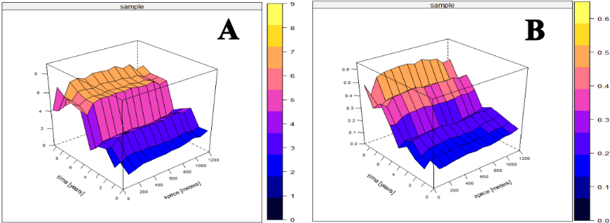
The space–time semivariograms (Figures 1 and 2) indicate only a modest rise with spatial lag, most evident at short distances. This points to a small spatial range: nearby points are correlated, whereas at larger separations variability is effectively random, consistent with a stable spatial structure.
Along the temporal axis (also in Figures 1 and 2), semivariance increases with time lag, showing that the chemical attributes become less similar as the interval grows. The temporal effect is stronger than the spatial one and is particularly marked for calcium and pH (Figures 1A and 1B). Phosphorus exhibits a gradual rise that levels off at roughly half the total temporal extent (Figure 2A). For magnesium and organic matter (Figures 2B and 2C), the increase is milder and concentrated in the initial time lags.
Analysis of the adjusted models and their parameters
The sample space-time semivariograms were adjusted by different spatial-temporal geostatistical models. The best fits were obtained with the sum-metric model for phosphorus (Figure 3A) and magnesium (Figure 3B), and with the simple sum-metric model for organic matter (Figure 3C), calcium (Figure 4A), and pH (Figure 4B). As noted by Heuvelink et al. (2012), these models help reduce uncertainty and allow separate interpretation of spatial, temporal, and joint components, though parameter estimation can be challenging given the number of parameters (Snepvangers et al., 2003). Prior work supports the effectiveness of models that incorporate spatial, temporal, and space–time terms for stochastic processes (Cesare et al., 2001; Snepvangers et al., 2003; Kilibarda et al., 2015; Monteiro et al., 2017).
These results show the importance of considering space-time variability beyond the purely spatial and temporal components for a more accurate adjustment of the model and, consequently, for obtaining more accurate results. The spatial-temporal models used in this study are formed by the purely spatial, purely temporal, and spatial-temporal components (joint). For each of these components, it is necessary to adjust by means of geostatistical models that best represent their behavior.
|
|---|
| Figure 1. Sample space-time semivariogram for: (A) Calcium; (B) pH. A steeper increase in the semivariogram is observed along the temporal axis than along the spatial axis, indicating greater variability and range of this component for both soil chemical elements. |
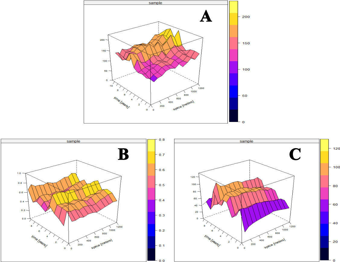
Figure 2. Sample space-time semivariogram for: (A) phosphorus; (B) magnesium; (C) organic matter. Phosphorus shows a gradual temporal increase and strong dependence, while magnesium and organic matter display smoother and more stable behavior. All three attributes exhibit short spatial ranges, indicating limited spatial continuity.
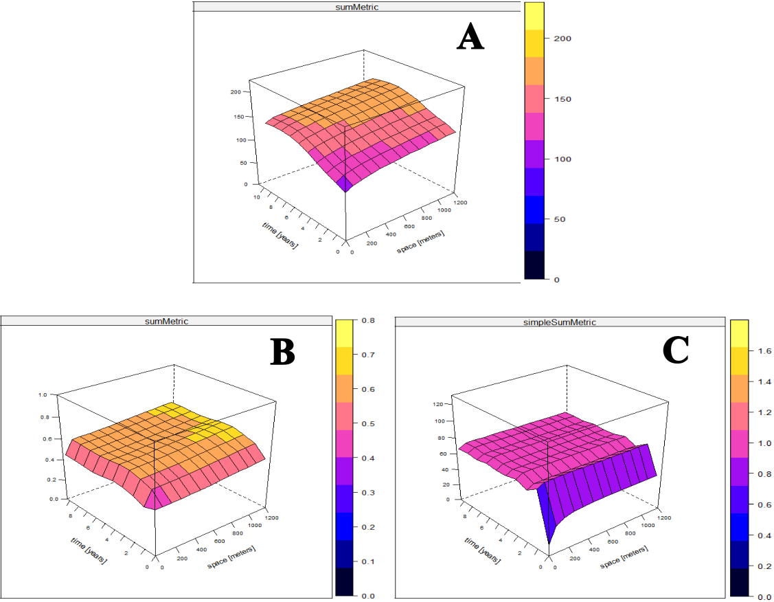
Figure 3. Fitted space–time models for (A) phosphorus, (B) magnesium, and (C) organic matter using the sum-metric and simple sum-metric approaches. The fitted surfaces show good agreement with the experimental data, separating spatial, temporal, and joint components.
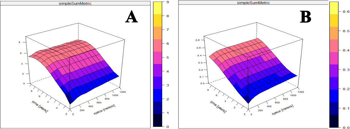
Figure 4. Fitted simple sum-metric models for (A) calcium and (B) pH. The fitted surfaces show good agreement with the experimental data, separating spatial, temporal, and joint components.
| Table 1. Spatio-temporal geostatistical parameters for the purely spatial component. | |||||
|---|---|---|---|---|---|
| Phosphorus | Magnesium | Calcium | pH | Organic Matter | |
| Model | Gaussian | Matérn k=2 | Wave | Spherical | Exponential |
| Nugget \(({\widehat{\varphi}}_{1})\) | 5.0 | 0.13 | 0.93 | 0.08 | 13.95 |
| Partial Sill \({(\widehat{\varphi}}_{2})\) | 4.01 | 0.14 | 0.44 | 0.05 | 5.01 |
| Sill (\({\widehat{\varphi}}_{1} + {\widehat{\varphi}}_{2})\) | 9.01 | 0.27 | 1.37 | 0.13 | 18.96 |
| Range (m) | 178 | 580 | 158 | 229 | 30 |
| RNE | 0.55 (md) | 0.48 (md) | 0.68 (md) | 0.61 (md) | 0.74 (md) |
| RNE: (\(\ {\widehat{\varphi}}_{1}/({\widehat{\varphi}}_{1} + {\widehat{\varphi}}_{2})\) relative nugget effect\(;\) md: moderate degree. | |||||
| Table 2. Spatio-temporal geostatistical parameters for the purely temporal component. | |||||
|---|---|---|---|---|---|
| Phosphorus | Magnesium | Calcium | pH | Organic Matter | |
| Model | Wave | Wave | Wave | Wave | Wave |
| Nugget \(({\widehat{\varphi}}_{1})\) | 7.0 | 0.08 | 0.93 | 0.08 | 13.95 |
| Partial Sill \({(\widehat{\varphi}}_{2})\) | 30.73 | 0.08 | 2.78 | 0.23 | 28.41 |
| Sill (\({\widehat{\varphi}}_{1} + {\widehat{\varphi}}_{2})\) | 37.73 | 0.16 | 3.71 | 0.31 | 42.36 |
| Range (year) | 5 | 2 | 5 | 6 | 1 |
| RNE | 0.18 (sd) | 0.50 (md) | 0.25 (sd) | 0.25 (sd) | 0.33 (md) |
| RNE: (\(\ {\widehat{\varphi}}_{1}/({\widehat{\varphi}}_{1} + {\widehat{\varphi}}_{2})\) relative nugget effect\(;\) md: moderate degree; sd: strong degree. | |||||
Analysis of the purely spatial component
When adjusting the purely spatial structure, it is observed that there is no specific model that best fits the spatial component of space-time semivariograms; Gaussian, exponential, wave, spherical, and Matérn models were selected as appropriate (Table 1). These models are usually used in studies describing the spatial dependence structure in soil chemical attributes (Dalposso et al., 2019; Guedes et al., 2020; Dal'Canton et al., 2023; Lorbieski et al., 2023; Maltauro et al., 2023). Fitted parameters indicate mostly moderate spatial dependence with ranges <230 m—i.e., <¼ of the maximum interpoint distance (~1,766 m)— this is an indication of how variability is restricted near regions within the field. Magnesium is the exception, with a range of ~590 m, suggesting broader spatial continuity relative to other attributes.
Another aspect to be considered in relation to spatial variability is its pattern over time. Across time lags (Figures 5–6), the spatial pattern is stable: semivariograms rise steeply at short distances and plateau early, regardless of temporal separation. This indicates a persistently small spatial range over the monitoring period. In other words, there is a rapid initial increase of variance of these semivariograms, quickly reaching a level that indicates a reduced radius of spatial dependence, regardless of the time distance between the samples.
Despite the common pattern, pH and calcium (Figures 5A–B) show higher contributions at the longest temporal lags (represented in the graphs with colors close to yellow)—i.e., larger sill–nugget differences— indicating an increase in the variability of samples separated by longer distances in time. This behavior indicates an increase in spatial variability over the years, caused by differences in sample values over time, however, as the range has changed little in different time lags, the increase in variability was restricted to regions near the sampling points. For phosphorus, magnesium, and organic matter (Figures 6A–C), contributions do not increase with time lag, indicating stability or minor temporal change.
Overall, the attributes exhibit short-range spatial dependence and localized variation; This behavior reveals an apparent randomness in spatial variability patterns in this area that may be associated with events with effects located within the field that affect the spatial distribution of these attributes on a local scale.
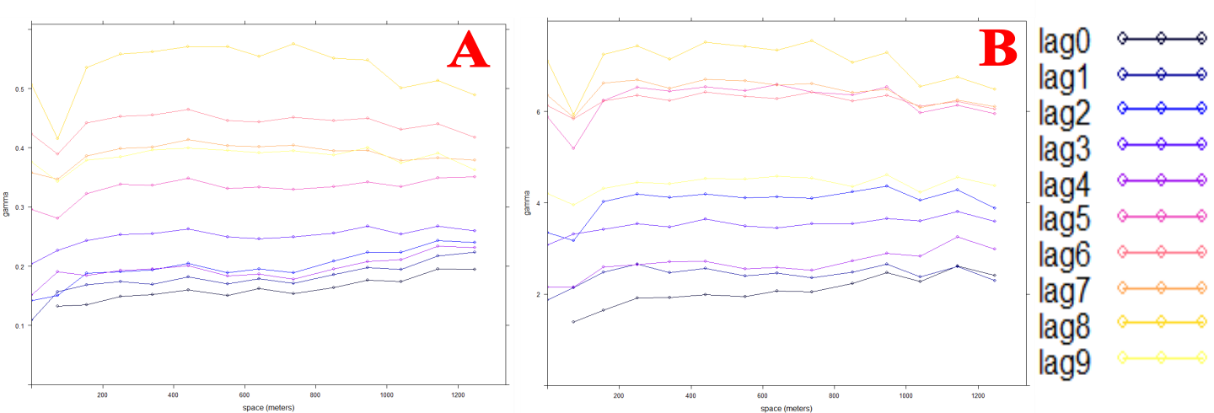
Figure 5. Sample semivariograms separated by temporal lags; A: pH, B: calcium. The lag considers the samples used according to the time interval between them. The number in the sequence indicates the time interval that separates the samples: lag0 includes all samples, lag1 includes all samples separated by one year, and so on. The curves remain similar across time lags, indicating stable short spatial ranges, while larger time intervals show higher variance levels, suggesting increasing temporal variability restricted to local areas.
| Table 3. Variances of the canonical pairs U and V and the correlation between them. | ||||
|---|---|---|---|---|
| Canonical Pairs | Variance | % Variance | % Accumulated Variance | Canonical Correlation |
| U1V1 | 0.995 | 62.97 | 62.97 | 0.997 |
| U2V2 | 0.585 | 37.02 | 100.00 | 0.765 |
| Table 4. Significance test of canonical pairs. | ||||||
|---|---|---|---|---|---|---|
| Canonical Function | Canonical Pairs | λ de Wilks | Chi-Square | chi-square density | df | p-Valor |
| 1 | (U1V1) | 0.002 | 24.678 | 18.307 | 10 | 0.006* |
| 2 | (U2V2) | 0.415 | 3.517 | 9.487 | 4 | 0.475 |
| Table 5. Canonical Loadings for the First Canonical Function (U1V1). | |
|---|---|
| Independent Variables | |
| Variables | Canonical Loadings |
| Average daily precipitation | -0.80 |
| Average daily temperature | 0.11 |
| Dependent Variables | |
| Variables | Canonical Loadings |
| Phosphorus | 0.39 |
| Organic Matter | 0.33 |
| Calcium | 0.41 |
| pH | 0.08 |
| Magnesium | 0.23 |
A related study in the same area (Lorbieski et al., 2023) identified zones with similar characteristics from spatial variability patterns and reported that, although soil chemical attributes varied, the variation was confined to a range that did not affect productivity. This likely reflects site management under technical supervision typical of a commercial field. Consistent with this, Kayad et al. (2021) note that both management and environmental factors shape spatial and temporal variability; Freddi et al. (2006) point to management as the primary driver; and Khan et al. (2020) show that well-implemented practices can mitigate such variability.
Other studies support these findings. Klic et al. (2012) showed that soil preparation in cultivated areas alters properties and tends toward homogenization relative to uncultivated sites. Liu et al. (2009) likewise reported reduced spatial variability of soil chemical properties in an irrigated rice system after two decades of improved management. These results align with Carvalho et al. (2003), who argue that spatial variability reflects both intrinsic controls (parent material, texture) and extrinsic drivers linked to management (e.g., fertilization, liming).
Analysis of the purely temporal component
As for the temporal component, the wave model provided the best fit (Table 2). The sample space–time semivariograms (Figures 1–2) show periodic behavior along the temporal axis, and the wave model captures this non-monotonic, oscillatory pattern (Andriotti, 2009; Chilès and Delfiner, 2012). The model is also widely used for climate-related variables (Isaaks and Srivastava, 1989; Cressie, 2015; Gamero et al., 2020). Because temporal variability in soil chemistry is largely climate-driven
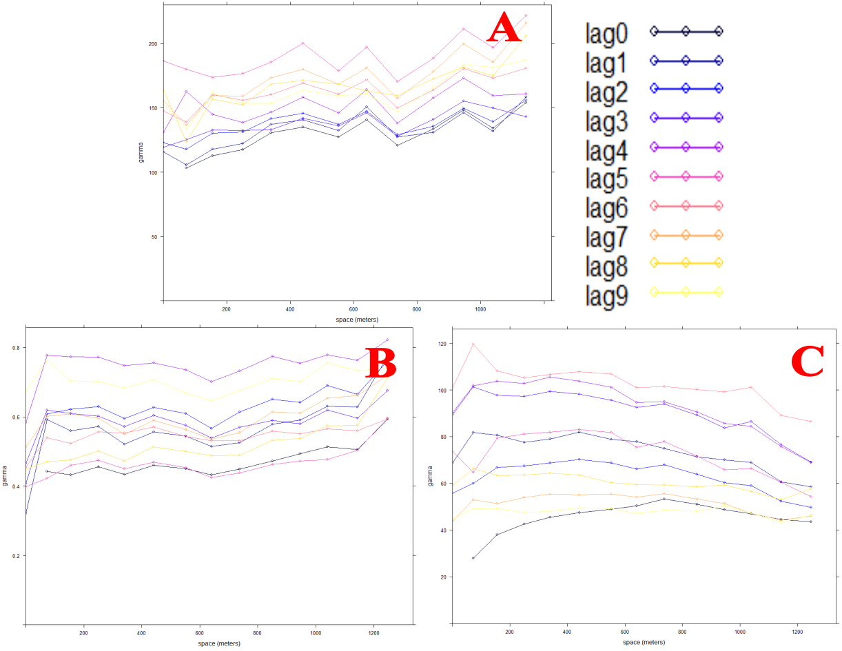
Figure 6. Sample semivariograms separated by temporal lags; A: phosphorus, B: magnesium; C: organic matter. The lag considers the samples used according to the time interval between them. The number in the sequence indicates the time interval that separates the samples: lag0 includes all samples, lag1 includes all samples separated by one year, and so on. The consistent curve patterns and early plateaus across lags indicate spatial stability and minimal change in variability through time.
| Table 6. Spatio-temporal geostatistical parameters for the spatio-temporal component (joint). | |||||
|---|---|---|---|---|---|
| Phosphorus | Magnesium | Calcium | pH | Organic Matter | |
| Model | Matérn k=0.3 | Exponential | Exponential | Matérn k=0.3 | Matérn k=0.3 |
| Nugget \(({\widehat{\varphi}}_{1})\) | 95.66 | 0.30 | 0.93 | 0.08 | 13.95 |
| Partial Sill \({(\widehat{\varphi}}_{2})\) | 73.91 | 0.01 | 1.49 | 0.08 | 25.76 |
| Sill (\({\widehat{\varphi}}_{1} + {\widehat{\varphi}}_{2})\) | 169.57 | 0.31 | 2.42 | 0.16 | 39.71 |
| Range (m) | 3915 | 1962 | 964 | 1447 | 149 |
| RNE | 0.56 (md) | 0.96 (wd) | 0.38 (md) | 0.50 (md) | 0.35 (md) |
| StAnis | 0.10 | 0.11 | 3.66 | 0.63 | 3.38 |
| RNE: (\(\ {\widehat{\varphi}}_{1}/({\widehat{\varphi}}_{1} + {\widehat{\varphi}}_{2})\) relative nugget effect\(;\) md: moderate degree; wd: weak degree; StAni: spatio-temporal anisotropy. | |||||
(Heuvelink and van Egmond, 2010; Basso et al., 2012; Liu et al., 2016), these features justify the superior fit of the wave model to the temporal structure.
The temporal patterns seen in the experimental semivariograms (Figures 1–2) and fitted models (Figures 3–4) are consistent with the model parameters (Table 2). The purely temporal component shows moderate to strong dependence, with temporal ranges of 1–6 years. Phosphorus, calcium, and pH exhibit the highest dependence and longest ranges—about 6 years for pH and 5 years for phosphorus and calcium—indicating gradual changes that persist across multiple years. The remaining attributes display shorter ranges and weaker dependence, suggesting less temporal correlation and more year-to-year variability.
This temporal behavior is consistent with prior work showing that soil chemical attributes are generally not temporally stable (Gavioli et al., 2016; Cammarano et al., 2020). Several studies report year-to-year changes: Ferraz et al. (2012) found interannual variation in soil phosphorus and potassium; Cox et al. (2003) observed that soil fertility varied annually across fields; and Liu et al. (2009) documented increases in organic carbon, total nitrogen, and available phosphorus, along with a marked decline in available potassium, linked to imbalanced N–P–K fertilization.
Heuvelink and Egmond (2010) argue that rainfall can produce greater temporal than spatial variation because it tends to affect the whole field while changing markedly over time. To examine this, we related climatic variables to soil chemical attributes using canonical correlation analysis (CCA). The CCA results (Table 3; Figure 7) indicate that the first canonical
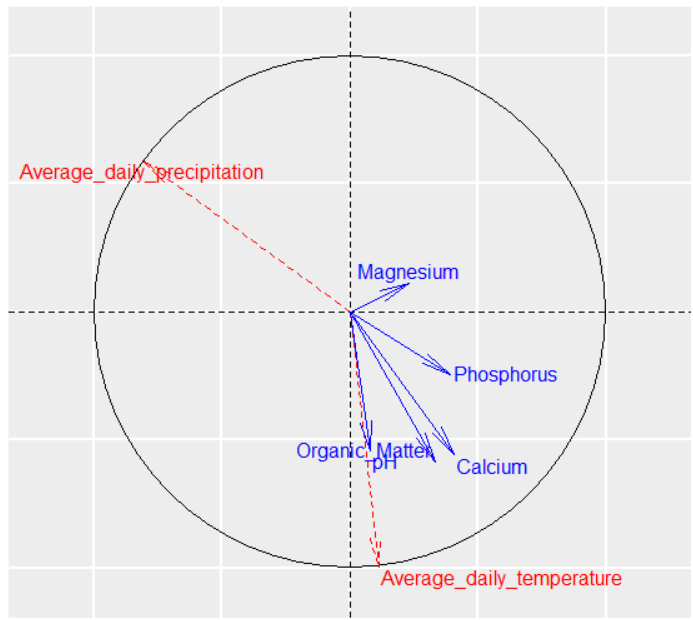
Figure 7. Biplot of the canonical correlation between climatic variables and soil chemical attributes. Precipitation shows a strong negative association with soil attributes, while temperature has a weaker positive relationship, indicating that rainfall is the main climatic driver of soil chemical variability.
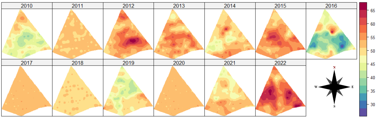
Figure 8. Map of soil organic matter content between the years 2010 and 2022. It shows more pronounced year-to-year variations than the other soil chemical attributes, indicating that changes in organic matter are mainly the result of specific annual events, either climatic or management-related.
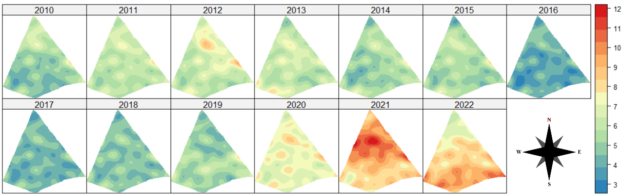
Figure 9. Map of soil calcium content between the years 2010 and 2022. Lower concentrations are observed between 2015–2017 and higher values from 2020–2022, corresponding to liming cycles and the longer temporal ranges identified in the model.
pair (U1–V1) explains 99.5% of variance in its dependent canonical variate, representing about 63% of the total variance considered in the analysis. The second pair (U2–V2) accounts for 0.585, or roughly 37% of the total. The canonical correlation for the first pair is 0.997, indicating a very strong association between the canonical functions; the second pair is also strong but lower.
According to the significance tests (Table 4), only the first canonical pair (U1–V1) was significant (p < 0.05). This indicates that variation in the soil‐attribute set, for this pair, is explained primarily by the climate set rather than random error. The higher Wilk λ for the second pair (U2–V2) suggests its result is more likely accidental under this model. Therefore, interpretation is restricted to U1–V1.
Table 5 shows that daily mean precipitation has the largest loading among the climatic variables for U1–V1, with a negative sign—i.e., higher precipitation is associated with lower values of the soil chemical attributes. Mean daily temperature has a positive loading but a smaller magnitude, indicating a weaker, direct association with the soil attribute set.
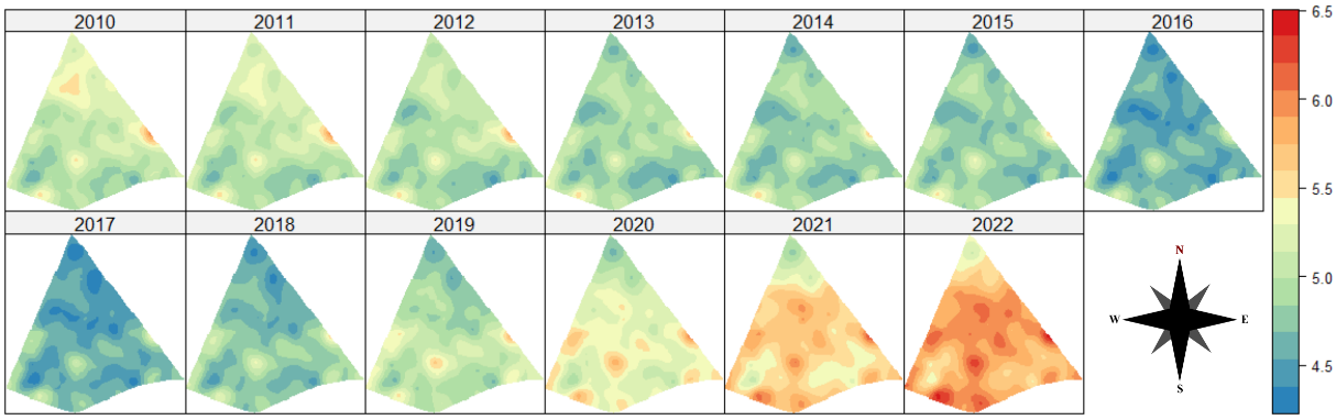
Figure 10. Soil pH map between the years 2010 and 2022. Lower values are observed between 2015–2017 and higher ones between 2020–2022, showing that the pH distribution mirrors the calcium pattern and confirms the positive correlation and shared temporal trend associated with soil acidity correction practices.
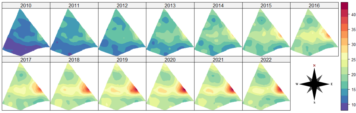
Figure 11. Map of soil phosphorus content between the years 2010 and 2022. A persistent high-concentration zone appears in the central-western region, with a slight gradual increase over the years, consistent with the low solubility and mobility of phosphorus in soil.
Calcium, phosphorus, and organic matter show the strongest association with daily mean precipitation (Table 5): higher precipitation is linked to lower values of these attributes. Mean daily temperature also relates to the soil set but weaklier.
This pattern appears in the CCA biplot (Figure 7): precipitation vectors oppose the soil-attribute vectors (inverse relationship), while temperature aligns in the same general direction (direct but weaker association), consistent with a smaller and possibly incidental effect.
Intense rainfall accelerates nutrient loss via leaching and surface runoff, affecting multiple soil chemicals. In irrigated maize, nitrate leaching increases late in the crop cycle (Silva et al., 2009). Simulated storms have shown losses up to 60 kg ha⁻¹ of potassium from surface layers (Rosolem et al., 2006), and greater precipitation enhances calcium and magnesium leaching, contributing to acidification (Gelybó et al., 2018). Under varied management systems, heavy‐rainfall simulations also drive N, P, and K losses through runoff (Melo et al., 2024). Rising temperatures, in turn, can intensify organic matter mineralization: soils with higher organic C exposed to warmer conditions released more CO₂ over time, indicating accelerated decomposition and increased availability of soil substrates (Yu et al., 2022).
Intense rainfall increases nutrient losses via leaching and surface runoff, affecting multiple soil elements. In irrigated maize, nitrate leaching rises late in the crop cycle (Silva et al., 2009). Simulated storms have shown losses up to 60 kg ha⁻¹ of potassium from surface layers (Rosolem et al., 2006), and greater precipitation enhances calcium and magnesium leaching, contributing to acidification (Gelybó et al., 2018). Under different management systems, heavy-rainfall simulations also drive N, P, and K losses through runoff (Melo et al., 2024). Rising temperatures can intensify organic-matter mineralization: soils richer in organic carbon exposed to warmer conditions released more CO₂ over time, indicating accelerated decomposition and greater substrate availability (Yu et al., 2022).
In summary, climate explains a substantial share of the variability in soil chemical attributes, but not all of it; management practices, cultivar characteristics, and other site factors also contribute. This aligns with Basso et al. (2012), who argue that temporal variability is driven mainly by non-stationary drivers such as climate and yearly crop choices.
Space-time component (joint)
The joint space–time component was best fitted by Matérn models with k = 0.3 (Table 6). Such a small smoothness parameter implies a relatively irregular process with rapid variation at short lags (Minasny and McBratney, 2007). Spatial–temporal model parameters (Table 6) show weak to moderate dependence across the soil chemical attributes, evidencing interaction between spatial and temporal components. Phosphorus and pH show the strongest space–time interaction (moderate dependence) and comparatively larger ranges than the other attributes.
Another relevant aspect related to the joint variability is the space-time anisotropy (Table 6). The values below 1 attributed to phosphorus, magnesium and pH suggest a more robust temporal correlation in the interaction between the levels of these soil chemical attributes. On the other hand, calcium and organic matter exhibit values higher than 1, indicating a more pronounced spatial correlation in this context of interaction (Gasch et al., 2015).
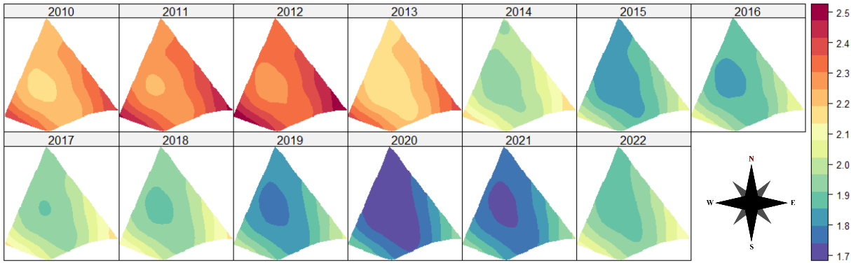
Figure 12. Map of soil magnesium content between the years 2010 and 2022. The maps reveal a gradual decline in magnesium levels throughout the study period, with decreasing concentrations after 2015.
Analysis of the different soil chemical attributes
By conducting a specific analysis for each soil chemical attribute, we found that organic matter, although showing moderate dependence across all evaluated components, also exhibited limited ranges in each of them (Tables 1, 2, and 6). In other words, autocorrelation among the observed values is confined to periods close to the observation year, given the one-year temporal window. This suggests that, overall, variability in this soil attribute is mostly random across the study area, with a stronger temporal component. This is clearer in Figure 8, which shows more abrupt year-to-year contrasts and less smooth change than the other chemical attributes analyzed. In sum, the values appear to be driven by year-specific events affecting this attribute.
Among the main factors contributing to the variability of soil organic matter are soil management and climatic conditions. Several studies in literature support this view. Liu et al. (2020) reported that the variability of organic soil matter is sensitive to human practices such as organic fertilization and land use changes. Similarly, Hu et al. (2018) found that both natural factors, including climate and topography, and human activities, such as land use and fertilization, influence its spatial distribution. According to Shi et al. (2019), dynamic human activities over short periods—such as land use, fertilization, soil preparation, and cropping systems—have a strong impact on the dynamics of soil organic matter.
Calcium, phosphorus, and pH showed the highest degrees of temporal dependence, along with moderate spatial dependence and limited space–time interaction across attributes (Tables 1, 2, and 6). Although pH is often reported to vary little (Amado et al., 2009; Ou et al., 2017), we observed the opposite. A likely explanation is its linkage to calcium: calcium amendments (e.g., liming) neutralize acidity and raise pH, so increases in calcium tend to increase pH (Pauletti et al., 2014). This relationship is evident in the maps (Figures 9 and 10), which it is possible to see lower values for both calcium and pH in 2015–2017 and higher values in 2020–2022. The same pattern appears in the sample and fitted semivariograms (Figures 1 and 4) and in the model parameters (Tables 1, 2, and 6).
Regarding phosphorus, a key property noted by Shen et al. (2011) is its low solubility and mobility in soil. The strong temporal dependence observed here may reflect this property, implying slow dispersion over time. Figure 11 supports this pattern: a high-concentration zone in the central-western portion of the area persists across years, with a slight, gradual increase over time.
Magnesium showed moderate spatial and temporal dependence; spatially, it showed a great dependence radius, among all attributes. In Figure 12, a gradual decline in magnesium over the study years is evident, and from 2015 onward the pattern becomes clearer, with values decreasing from north to south across the area.
Similar patterns have been reported in the literature. Stipek et al. (2004) documented spatial and temporal variation in soil magnesium, noting low spatial variability but moderate to strong spatial dependence and little temporal change. They concluded that, despite shifts in spatial variability, the mean and median remain stable, indicating consistent nutrient levels over time.
Materials and Methods
Area of study
The study used data on soil chemical attributes, including calcium (Ca) (cmolc dm⁻³), phosphorus (P) (mg dm⁻³), organic matter (OM) (g dm⁻³), pH (CaCl₂), and magnesium (Mg) (cmolc dm⁻³), collected before soybean sowing over nine crop years (2010–2022). Sampling was conducted in a 167.35-hectare commercial area in Cascavel, Paraná, Brazil (24.95° S, 53.37° W) at an average elevation of 650 m (Figure 13). The soil is classified as a Typical Dystroferric Red Latosol with a clayey texture (Santos et al., 2018). According to the Köppen classification, the region has a mesothermal, super-humid temperate climate (Cfa), with a mean annual temperature of 21 °C (Aparecido et al., 2016) and average precipitation of about 1,800 mm (Cattanêo et al., 2016).
Climatic anomalies varied during the study period. Extreme rainfall events linked to the 2015–2016 El Niño were recorded in Paraná (Montanher et al., 2023), and monthly precipitation in Cascavel showed significant correlation with the Oceanic Niño Index (ONI), indicating sensitivity to ENSO events (Pedron et al., 2023). Conversely, La Niña episodes were associated with below-average rainfall and severe droughts in southern Brazil (Grimm et al., 2020), confirming the influence of ENSO cycles on precipitation variability in the region.
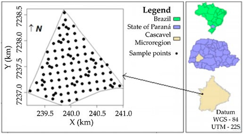
Figure 13. Representation of the plot with the sampling points (Flat coordinate system, UTM projection, zone 22 South, SIRGAS 2000 datum).
The sampling design included 102 points distributed by the lattice plus close pairs method (Figure 13), providing uniform spatial coverage (Maltauro et al., 2023). The layout comprised a regular grid with 141 m spacing between points, complemented by additional pairs at 75 and 50 m to capture finer-scale variability. All points were georeferenced using GPS with the WGS84 datum and UTM projection (Maltauro et al., 2025).
No data were collected in 2011, 2017, 2018, and 2020. The area is managed under no-tillage with annual rotation between soybean and off-season maize, and soil correction is performed as needed based on annual analyses and thematic maps.
Spatial-temporal geostatistical analysis
The spatial–temporal variability of soil variables was analyzed using the space–time semivariogram derived from Equation 1 and its corresponding fitted geostatistical model. The estimated space–time semivariance function, \({\widehat{\gamma}}_{st}\left( \mathbf{h},\mu \right)\), is a generalization of the classical spatial formulation proposed by Matheron (1989) (Eq. 1; Montero et al., 2015):
| \(\ {\widehat{\gamma}}_{st}\left( \mathbf{h},\mu \right)\ = \frac{1}{N\left( \mathbf{h},u \right)}\sum_{i = 1}^{N\left( \mathbf{h},u \right)}\left\lbrack Z\left( \mathbf{s}_{\mathbf{i}},t_{i} \right) - Z\left( \mathbf{s}_{\mathbf{j}},t_{j} \right) \right\rbrack^{2}\), | Eq. 1 |
|---|
where \(Z(s_{i},t_{i})\) and \(Z(s_{j},t_{j})\)are pairs of observed values of the georeferenced variable in space and time, separated by an omnidirectional spatial lag \(\mathbf{h} = \mathbf{s}_{i} - \mathbf{s}_{j}\), with \(\mathbf{s}_{i},\mathbf{s}_{j} \in D \subset \mathbf{R}^{2}\), and a temporal lag \(u = t_{i} - t_{j}\), with \(t_{i},t_{j} \in T \subset \mathbb{R}\). \(N(\mathbf{h},u)\) represents the number of data pairs separated by the space–time lag \((\mathbf{h},u)\).
In this framework, semivariograms were computed for different time intervals. The estimation of the space–time semivariogram (Eq. 1) combines spatial and temporal distances (Matheron, 1989). The semivariance is considered purely spatial when temporal distance equals zero \((\mathbf{h},0)\) (Figure 14A), purely temporal when spatial distance equals zero \((0,u)\) (Figure 14B), and space–time when both distances differ from zero (Figure 14C) (Montero et al., 2015).
To model space–time dependence, five semivariance models were evaluated Initially we have the sum model \(\gamma_{so}(\mathbf{h},u)\) (Eq. 2) and the sum–product model \(\gamma_{sp}(\mathbf{h},u)\) (Eq. 3), both represented as a sum or product of purely spatial \(\gamma_{s}(\mathbf{h})\) and purely temporal \(\gamma_{t}(u)\) components. The metric model \(\gamma_{m}(\mathbf{h},u)\) (Eq. 4) combines spatial, temporal, and space–time distances through an anisotropy correction that equates spatial and temporal units, using the metric \(\sqrt{\parallel \mathbf{h} \parallel^{2} + c^{2} \mid u \mid^{2}}\)in the stationary case, where c is the anisotropy correction factor. Finally, the simple sum–metric \(\gamma_{sm}(\mathbf{h},u)\) (Eq. 5) and sum–metric \(\gamma_{ssm}(\mathbf{h},u)\) (Eq. 6) models combine the sum and metric formulations. The distinction between them lies in whether the nugget effect (nug) is assigned the same value across all components (spatial, temporal, and space–time) during model fitting (Montero et al., 2015; Viana et al., 2019).
| \[\gamma_{so}\left( \mathbf{h},u \right) = \gamma_{s}\left( \mathbf{h} \right) + \gamma_{t}(u),\ \ \left( \mathbf{h},\mu \right) \in \ \mathbf{D}\ X\ T\ ;\] | Eq. 2 |
|---|---|
| \[\gamma_{sp}\left( \mathbf{h},u \right) = \left( k_{1}{sill}_{t} + k_{2} \right)\gamma_{s}\left( \mathbf{h} \right) + \left( k_{1}{sill}_{s} + k_{3} \right)\gamma_{t}(u) - k_{1}\gamma_{s}\left( \mathbf{h} \right)\gamma_{t}(u),\ \ \left( \mathbf{h},\mu \right) \in \mathbf{D}\ X\ T\ ;\] | Eq. 3 |
| \[\gamma_{m}\left( \mathbf{h},u \right) = \gamma_{st}\left( \sqrt{\left\| \mathbf{h} \right\|^{2} + c^{2}|u|^{2}} \right),\ \ \left( \mathbf{h},\mu \right) \in \mathbf{\ }\mathbf{D}\ X\ T;\ \] | Eq. 4 |
| \[\gamma_{sm}\left( \mathbf{h},u \right) = \gamma_{s}\left( \mathbf{h} \right) + \gamma_{t}(u) + \gamma_{st}\left( \sqrt{\left\| \mathbf{h} \right\|^{2} + c^{2}|u|^{2}} \right),\ \ \left( \mathbf{h},\mu \right) \in \ \mathbf{D}\ X\ T;\ \] | Eq. 5 |
| \[\gamma_{ssm}\left( \mathbf{h},u \right) = nug + \gamma_{s}\left( \mathbf{h} \right) + \gamma_{t}(u) + \gamma_{st}\left( \sqrt{\left\| \mathbf{h} \right\|^{2} + c^{2}|u|^{2}} \right)\ \ \left( \mathbf{h},\mu \right) \in \ \mathbf{D}\ X\ T\ ;\] | Eq. 6 |
in which \(\gamma_{s}(.)\) \(\gamma_{t}(.)\) , and \(\gamma_{st}(.)\) are respectively the purely spatial, purely temporal and joint semivariance functions; \({sill}_{s}\) is the level parameter of \(\gamma_{s}(.)\) and \({sill}_{t}\) is the level parameter\(\ \gamma_{t}(.)\)of ; the parameter 𝑘 is the proportionality coefficient among the semi variance functions, \(k_{1} \geq 0,\ \ k_{2} \geq 0\ e\ k_{3} \geq 0\) are constant that ensure the validity of \(\gamma_{sp}\), and the estimation of their values is described by Viana et al. (2019). The space-time anisotropy correction factor \(c\) is used to merge distance in space with distance in time. The \(nug\) parameter is the value for the nugget effect that will be considered in all components (spatial, temporal and space-time) of the simple sum-metric model.
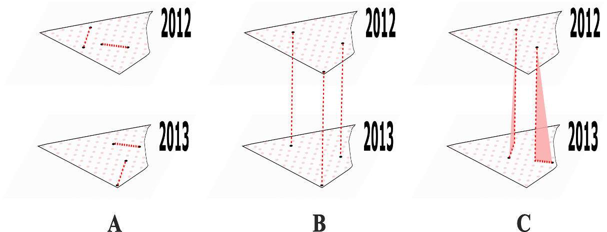
Figure 14. Combination of space-time distances; in the examples, the following were considered: (A) purely spatial: considering spatial distance with X and temporal distance with 0 years (X, 0); (B) purely temporal: considering spatial distance with 0 and temporal distance with T (0, T); (C) space-time: considering spatial distance with X and temporal distance with T (X, T). The figure visually illustrates the conceptual basis of the space–time semivariogram (Equation 1), showing how the spatial, temporal, and joint components are interconnected in modeling the dependence among soil observations over time and across the studied area.
The parameters of the geostatistical models were estimated using the ordinary least squares (OLS) method. Model performance was evaluated through the mean square error (MSE) statistic, and the model with the lowest MSE was selected as the best fit. This approach is commonly applied to assess interpolation accuracy, where lower MSE values indicate higher predictive precision (Viana et al., 2019).
The purely spatial, purely temporal, and space–time components of each semivariance model were fitted using one-dimensional isotropic semivariograms (Viana et al., 2019). The models applied included the exponential, Gaussian, Matérn, and wave models (Isaaks and Srivastava, 1989; Uribe-Opazo et al., 2012; Cressie, 2015).
To better understand the behavior of the soil chemical attributes analyzed, thematic maps were generated for all study years. According to Uribe-Opazo et al. (2023), such maps support improved field management, enabling the delineation of management zones and localized input application, among other uses. Data interpolation and map generation were performed using the ordinary space–time kriging (STOK) method (Eq. 7), whose equations are analogous to those of standard kriging (Viana et al., 2019):
| \[{\widehat{Z}}^{'}\left( \mathbf{s}_{0},t_{0} \right) = \sum_{\left\{ i:\mathbf{s}_{i},t_{i}\epsilon\mathbf{S}_{0} \right\}}^{}{\lambda_{i}Z^{'}\left( \mathbf{s}_{i},t_{i} \right)}\] | Eq. 7 |
|---|
where \(\mathbf{S}_{0}\)denotes the set of sampling points within the search neighborhood of the prediction location, \({\widehat{Z}}^{'}(\mathbf{s}_{0},t_{0})\) is the predicted value at an unsampled location and time, \(Z^{'}(\mathbf{s}_{i},t_{i})\) are the observed neighboring values, and \(\lambda_{i}\)are the corresponding space–time kriging weights (Varouchakis, 2018).
All model fitting and space–time analyses were performed in R (R Core Team, 2024) using the gstat (Pebesma, 2004) and spacetime (Pebesma, 2012) packages.
Analysis of the relationship between climate variables and chemical attributes of the soil
To assess the linear relationships and degrees of association between climatic variables and soil chemical attributes, a canonical correlation analysis (CCA) was performed. Canonical correlation is a multivariate statistical method that evaluates the relationship between two variable sets by identifying linear combinations within each set that maximize their mutual correlation. In essence, it reveals global patterns of association between the sets, indicating how they relate as a whole (Hair et al., 2009).
This analysis aimed to examine the associations between the climatic variables—mean daily precipitation (mm) and average daily temperature (°C)—and the soil chemical attributes: calcium (cmolc dm⁻³), phosphorus (mg dm⁻³), organic matter (g dm⁻³), pH, and magnesium (cmolc dm⁻³). The criterion for retaining canonical pairs was based on Wilks’ lambda and the significance test (p < 0.05) (Hair et al., 2009).
Climatic data were obtained from the NASA Langley Research Center’s POWER Project, funded by the NASA Earth Science/Applied Science Program. Data were freely available online and covered, for each crop season, the period from August of one year to August of the following year—the month in which soil sampling was conducted.
Conclusion
The chemical attributes of the soil exhibited greater variability over time than across space, as indicated by the fitted geostatistical models, in which the temporal component showed higher contribution, range, and degree of dependence. This pattern may be associated with climatic anomalies during the study period, such as variations in rainfall in the Cascavel region. Spatial dependence was restricted to short distances, with variability increasing as the sampling points became farther apart. The management practices adopted in the area, including no-tillage, annual rotation between soybean and off-season maize, and soil correction based on annual technical evaluations, likely contributed to the spatial stabilization of soil attributes over time. Overall, the short ranges and moderate dependencies observed indicate local spatial variability primarily influenced by management practices, while temporal patterns reflect both residual management effects and responses to climatic conditions. Although of smaller magnitude, the space–time interaction suggests that variability cannot be fully explained when spatial and temporal components are analyzed independently.
The results demonstrate that space–time geostatistics is an effective tool for analyzing the joint spatial and temporal variability of soil attributes. This approach enables the identification of stable patterns that support site-specific management, optimize input use, and reduce losses from processes such as leaching.
Acknowledgements
Thanks to the support of the Coordination for the Improvement of Higher Education Personnel - CAPES, funding code 001, CNPq and Applied Statistics Laboratories (LEA) and Space Statistics (LEE), UNIOESTE.
References
Amado TJC, Pes LZ, Lemainski CL, Schenato RB (2009) Atributos químicos e físicos de Latossolos e sua relação com os rendimentos de milho e feijão irrigados. Rev Bras Cienc Solo. 33: 831-843.
Andriotti JLS (2009) Fundamentos de Estatística e Geoestatística. v.3. Unisinos, São Leopoldo.
Aparecido LEO, Rolim GS, Richetti J, Souza PS, Johann JA. Köppen (2016) Thornthwaite and Camargo climate classifications for climatic zoning in the State of Paraná, Brazil. Cienc Agrotec. 40:405-417. https://doi.org/10.1590/1413-70542016404003916.
Basso B, Fiorentino C, Cammarano D, Cafiero G, Dardanelli J (2012) Analysis of rainfall distribution on spatial and temporal patterns of wheat yield in Mediterranean environment. Eur J Agron. 41:52-65.
Bernardi AC, Bettiol GM, Grego CR, Andrade RG, Rabello LM, Inamasu RY (2017) Ferramentas de agricultura de precisão como auxílio ao manejo da fertilidade do solo. Cadernos de Ciênc. & Tecnol. 32(1/2):211-227.
Cammarano D, Zha H, Wilson L, Li Y, Batchelor WD, Miao Y (2020) A remote sensing-based approach to management zone delineation in small scale farming systems. Agron. 10(11):1767.
Carvalho MP, Takeda EY, Freddi OS (2003) Variabilidade espacial de atributos de um solo sob videira em Vitória Brasil (SP). Rev Bras Cienc Solo. 27:695-703.
Cattanêo AJ, Stangarlin JR, Bassegio D, Santos RF (2016) Crambe affected by biological and chemical seed treatments. Bragantia. 75(3): 292–298. DOI: 10.1590/1678-4499.565.
Cesare L, Myers DE, Posa D (2001) Estimating and modeling space–time correlation structures. Stat Prob Lett. 51(1):9-14.
Chilès JP, Delfiner P (2012) Geostatistics: modeling spatial uncertainty. Vol. 713. John Wiley & Sons, New Jersey.
Cox MS, Gerard PD, Wardlaw MC, Abshire MJ (2003) Variability of selected soil properties and their relationships with soybean yield. Soil Sci. Soc. Am. J. 67(4):1296-1302.
Cressie NAC (2015) Statistics for Spatial Data. rev. ed. John Wiley & Sons, New York.
Dalposso GH, Uribe-Opazo MA, Johann JA, Bastiani FD, Galea M (2019) Geostatistical modeling of soybean yield and soil chemical attributes using spatial bootstrap. Eng. Agríc. 39:350-357.
Dal'Canton LE, Maltauro TC, Guedes LPC, Uribe-Opazo MA, Cima EG (2023) Bivariate spatial correlation between soil attributes and soybean productivity in an agricultural area with Dystroferric Red Latosol. Aust J Crop Sci. 17(1):20-ii.
Daunoras J, Kačergius A, Gudiukaitė R. (2024). Role of soil microbiota enzymes in soil health and activity changes depending on climate change and the type of soil ecosystem. Biology, 13(2), 85.
De Bastiani F, Galea M, Cysneiros AHMA, Uribe-Opazo MA (2017) Gaussian spatial linear models with repetitions: An application to soybean productivity. Spat Stat. 21:319-335.
Ferraz GAS, Silva FMD, Carvalho LC, Alves MDC, Franco BC (2012) Variabilidade espacial e temporal do fósforo, potássio e da produtividade de uma lavoura cafeeira. Eng. Agríc. 32:140-150.
Freddi OS, Carvalho MP, Veronesi Júnior V, Carvalho GJ (2006) Produtividade do milho relacionada com a resistência mecânica à penetração do solo sob preparo convencional. Eng. Agríc. 26:113-121.
Gamero P, Uribe-Opazo MA, De Bastiani F, Johann JA, Guedes LPC (2020) Variabilidade espacial da precipitação no cultivo de milho segunda safra no Paraná utilizando o modelo Wave. Irriga. 25(3):521-536.
Gasch CK, Hengl T, Gräler B, Meyer H, Magney TS, Brown DJ (2015) Spatio-temporal interpolation of soil water, temperature, and electrical conductivity in 3D+ T: The Cook Agronomy Farm data set. Spat. Stat. 14:70-90.
Gavioli A, de Souza EG, Bazzi CL, Guedes LPC, Schenatto K (2016) Optimization of management zone delineation by using spatial principal components. Comput Electron Agric. 127:302-310.
Gelybó G, Barna G, Farkas C, Tóth É, Szabó B, Mészáros I (2018) Potential impacts of climate change on soil properties. Agrok. és Talajt. 67(2): 203–216.
Guedes LP, Bach RT, Uribe-Opazo MA (2020) Nugget effect influence on spatial variability of agricultural data. Eng. Agríc. 40:96-104.
Grimm AM, Almeida AS, Beneti CAA, Leite EA (2020) The combined effect of climate oscillations in producing extremes: the 2020 drought in southern Brazil. Rev Bras Recur Hídric. 25: e48. DOI: 10.1590/2318-0331.252020200116.
Hair JF, Black WC, Babin BJ, Anderson RE, Tatham RL (2009) Análise multivariada de dados. Bookman, Porto Alegre.
Heuvelink GBM, Van Egmond FM (2010) Geostatistical Applications for Precision Agriculture. Springer, Berlin.
Heuvelink GB, Griffith DA, Hengl T, Melles SJ (2012) Sampling Design Optimization for Space‐Time Kriging. In: Spatio‐Temporal Design: Advances in Efficient Data Acquisition. Wiley, New Jersey. 9
Hu PL, Liu SJ, Ye YY, Zhang W, Wang KL, Su YR (2018) Effects of environmental factors on soil organic carbon under natural or managed vegetation restoration. Land Degrad. Dev. 29(3):387-397.
Isaaks EH, Srivastava RM (1989) Applied geostatistics. Oxford University Press, Oxford.
Judijanto L, Suparwata DO, Sarie F, Safruddin, Sutrisno E (2024) The Role of Soil Type and Environmental Conditions in Increasing Soybean Production. West Science Agro 2 (02): 56-62. https://doi.org/10.58812/wsa.v2i02.943.
Liu X, Zhang W, Zhang M, Ficklin DL, Wang F (2009) Spatio-temporal variations of soil nutrients influenced by an altered land tenure system in China. Geod. 152(1-2):23-34.
Liu XL, Fu XQ, Li Y, Shen JL, Wang Y, Zou GH, Wu YZ , Ma QM, Chen D, Wang C, Xiao RL, Wu JS (2016) Spatio-temporal variability in N2O emissions from a tea-planted soil in subtropical central China. Geosci Model Dev Discuss. [preprint]: 1-45.
Liu H, Li S, Zhou Y (2020) Spatial-temporal variability of soil organic matter in urban fringe over 30 years: a case study in Northeast China. Int J Environ Res Public Health. 17(1):292.
Lorbieski R, Guedes LPC, Uribe-Opazo MA, Kestring FBF (2023) Regionalization of an agricultural area by means of multivariate data and their relationship with soybean productivity. Aust J Crop Sci. 17(7):570-580.
Kayad A, Sozzi M, Gatto S, Whelan B, Sartori L, Marinello F (2021) Ten years of corn yield dynamics at field scale under digital agriculture solutions: A case study from North Italy. Comput Electron Agric. 185:106126.
Khan H, Acharya B, Farooque AA, Abbas F, Zaman QU, Esau T (2020) Soil and crop variability induced management zones to optimize potato tuber yield. Appl Eng Agric. 36(4):499-510.
Kilibarda M, Tadić MP, Hengl T, Luković J, Bajat B (2015) Global geographic and feature space coverage of temperature data in the context of spatio-temporal interpolation. Spat. Stat. 14:22-38.
Maltauro TC, Guedes LPC, Uribe-Opazo MA, Canton LE (2023) Multivariate spatial sample reduction of soil chemical attributes by means of application zones. Span J Agric Res. 21(2): e0205-e0205.
Maltauro TC, Uribe-Opazo MA, Guedes LPC, Galea M, Nicolis O (2025) Spatial–temporal variability of soybean yield using separable covariance structure. Agric. 15(1199): 1-21.
Matheron G (1989) Choice and Hierarchy of Models. In: Estimating and Choosing. Springer, Berlin.
Melo RF, Barbosa RS, Oliveira JF, Silva AC, Cunha JC (2024) Loss of nitrogen, phosphorus, and potassium through surface runoff under simulated rainfall in different soil management systems. Eng Sanit Ambient. 29: 1-5.
Minasny B, McBratney AB (2007) Spatial prediction of soil properties using EBLUP with the Matérn covariance function. Geod. 140(4): 324-336.
Montanher OC, Minaki C, Morais ES, Paula Silva J, Pereira P (2023) Geosystemic impacts of the extreme rainfall linked to the El Niño 2015/2016 event in Northern Paraná, Brazil. Appl. Sci. 13(17): 9678. DOI: 10.3390/app13179678.
Montero JM, Fernández-Avilés G, Mateu J (2015) Spatial and spatio-temporal geostatistical modeling and kriging. John Wiley & Sons, New York.
Monteiro A, Menezes R, Silva ME (2017) Modelling spatio-temporal data with multiple seasonalities: The NO2 Portuguese case. Spat. Stat. 22:371-387.
Noetzold R, de Carvalho Alves M, Marcos Goussain Júnior M, de Cássia Santos Goussain R (2019) Variabilidade Espacial Da Eficiência Do Uso De Potássio E Fósforo Na Cultura Da Soja. Eng. na Agric. 27(6): 529-541.
Ou Y, Rousseau AN, Wang L, Yan B (2017) Spatio-temporal patterns of soil organic carbon and pH in relation to environmental factors—A case study of the Black Soil Region of Northeastern China. Agric. Ecosyst. Environ. 245:22-31.
Pauletti V, Pierri LD, Ranzan T, Barth G, Motta ACV (2014) Efeitos em longo prazo da aplicação de gesso e calcário no sistema de plantio direto. Rev. Bras. Cienc. Solo. 38:495-505.
Pebesma EJ (2004) Multivariable geostatistics in S: the gstat package. Comput. Geosci. 30(7): 683-691.
Pebesma E (2012) spacetime: Spatio-temporal data in R. J Stat Softw. 51:1-30.
Pedron IT, Limberger L (2023) Sinal do fenômeno ENOS na precipitação pluvial da região oeste do Paraná. RAEGA - O Espaço Geográfico em Análise. 57: 114-135 DOI: 10.5380/raega.v57i0.89506.
R Development Core Team (2024) R: a language and environment for statistical computing. R Foundation for Statistical Computing, Vienna, Áustria. ISBN 3-900051 07-0. Available online: http://www.R-project.org/.
Resende AV, Coelho AM (2014) Muestreo para mapeo y manejo de la fertilidad del suelo. In: Mantovani EC, Magdalena C, Magdalena C, editors. Manual de agricultura de precisión.
Rosolem CA, Calonego JC, Foloni JSS (2006) Potássio no solo em consequência da adubação sobre a palha de milheto e chuva simulada. Pesq. Agropec. Bras. 41(6): 1033–1040
Santos HG, Jacomine PKT, Anjos LHC, Oliveira VA, Lumbreras JF, Coelho MR (2018) Sistema brasileiro de classificação de solos. 5. ed. rev. ampl. Embrapa, Brasília.
Shen J, Yuan L, Zhang J, Li H, Bai Z, Chen X, Zhang W, Zhang F (2011) Phosphorus dynamics: from soil to plant. Plant physiol. 156 (3): 997-1005.
Shi P, Zhang Y, Li P, Lia Z, Yu K, Ren Z, Xu G, Cheng S, Wang F, Ma Y (2019) Distribution of soil organic carbon impacted by land-use changes in a hilly watershed of the Loess Plateau, China. Sci. Total Environ. 652: 505-512.
Silva RC, Lima LA, Oliveira Filho EC, Frizzone JÁ (2009) Lixiviação de nitrato e amônio no perfil de Latossolo cultivado com milho irrigado. In: Congresso Nacional de Irrigação e Drenagem. 19.
Snepvangers JJJ, Heuvelink GBM, Huisman JÁ (2003) Soil water content interpolation using spatio-temporal kriging with external drift. Geod. 112(3-4): 253-271.
Štípek K, Vaněk V, Száková J, Černý J, Šilha J (2004) Temporal variability of available phosphorus, potassium and magnesium in arable soil. Plant Soil Environ. 50(12): 547-551.
Uribe-Opazo MA, Borssoi J, Galea M (2012) Influence diagnostics in Gaussian spatial linear models. J. of App. Stat. 39(3): 615–630.
Uribe-Opazo MA, Dalposso GH, Galea M, Johann JA, De Bastiani F, Cambillo Moyano EN, Grzegozewski DM (2023) Spatial variability of wheat yield using the gaussian spatial linear model. Aust. J. Crop Sci. 17(2): 179-189.
Varouchakis EA (2018) Spatiotemporal geostatistical modelling of groundwater level variations at basin scale: a case study at Crete’s Mires Basin. Hydrol Res. 49(4): 1131–1142.
Viana RSM, dos Santos GR, Moreira DS, Louzada JM, Rosa LMF (2019) O Uso da Geoestatística Espaço-Temporal na Predição da Temperatura Máxima do Ar. Rev Bras Geogr Fís. 12: 96-111.
Yang H, Song X, Zhao Y, Wang W, Cheng Z, Zhang Q, Cheng D (2021) Temporal and spatial variations of soil C, N contents and C: N stoichiometry in the major grain-producing region of the North China Plain. Plos One. 16(6): e0253160.
Yu H, Sui Y, Chen Y, Bao T, Jiao X (2022) Soil organic carbon mineralization and its temperature sensitivity under different substrate levels in the Mollisols of Northeast China. Life. 12(5): 712.
Zhuo Z, Xing A, Li Y, Huang Y, Nie C (2019) Spatio-temporal variability and the factors influencing soil-available heavy metal micronutrients in different agricultural sub-catchments. Sustain. 11(21): 5912.