Australian Journal of Crop Science
Article | https://doi.org/10.21475/ajcs.26.20.08.pne86
Submitted: 27 July 2025 | Revised: 21 October 2025 | Accepted: 05 June 2026
Pages 587-597
Machine learning in agriculture: Estimation of soybean yield in a Southern region of Brazil
Roney Peterson Pereira1, Luciana Pagliosa Carvalho Guedes1, Miguel Angel Uribe-Opaz1, André Luiz Brun2, Jean Carlos Cardoso3
1Western Paraná State University (UNIOESTE), Postgraduate Program in Agricultural Engineering, Cascavel, Paraná, Brazil
2Western Paraná State University (UNIOESTE), Computer Science Collegiate, Cascavel, Paraná, Brazil
3Federal University of Pernambuco (UFPE), Department of Statistics, Recife, Pernambuco, Brazil
Corresponding author: rppereira2@uem.br
Abstract: Agriculture is one of the most relevant economic sectors in Brazil, and corresponds to more than 20% of the Brazilian GDP. Currently, technologies applied to agriculture have provided the emergence of big data. In this context, machine learning techniques (MLT) are high-performance tools to understand, quantify and identify trends in agricultural areas. This study employed MLT to predict soybean yield in a commercial area located in the western region of Paraná State, Brazil, characterized by a humid subtropical climate (Cfa, Köppen), Dystroferric Red Latosol soil with clayey texture, and gently undulating relief, in order to optimize agricultural practices and maximize yields. The study area is characterized by a mesothermic and superhumid climate (Cfa, Köppen) and a Dystroferric Red Latosol with clayey texture. For this, information on soil chemical properties, rainfall and soybean yield were used, considering 7 crop years from 2012 to 2023. Random Forest (RF), Generalized Boosted Regression Modeling, Support Vector Regression (SVR), K-Nearest Regressor and Artificial Neural Networks (ANN) were compared. In this initial analysis, the RF and SVR models stood out as the most effective in predicting soybean yield, but did not present significant differences (5% probability) in the root of the mean quadratic error (RMSE) and the Mann-Whitney U test. It was identified that the soil’s iron and potassium content were the most important covariables associated with soybean yield. In a second analysis, the inclusion of monthly accumulated rainfall data during the soybean harvest led to improvements in soybean forecasting, as indicated by the metrics analyzed. The best results were obtained by the RF and KNR algorithms. Because the RF algorithm presented the lowest RMSE values (0.568 and 0.446) and the highest coefficient of determination (R²) (0.724 and 0.824) in both analyses, we applied the algorithm to the 2022/2023 crop year forecast and compared the results with actual crop year data. The results of this comparison are presented in Post-Plots and scatter plots. The results of this study have important implications, allowing more adequate forecasts of soybean yield and assisting farmers in decision making.
Keywords: covariables, yield optimization; forecasting models; agricultural yield, regression algorithms.
Abbreviations: Al_Aluminum content; ANN_Artificial Neural Networks; bag.fraction_subsampling fraction; Ca_Calcium content; Cfa: humid subtropical climate; Cu_Copper content; CV_coefficient of variation; Fe_iron content; GBM_Generalized Boosted Regression Modeling; GPS_Global positioning system; HAI3_Total potential acid; IncNodePurity_ purity of decision tree nodes; K_Potassium content; KNR_K-Nearest Regressor; LaRC_NASA Langley Research Center; Máx_maximum; Mg_magnesium content; Mín_minimum; MLs_Machine Learnings; Mn_Manganese content; mtry_number of variables splits; N_number of trees; P_phosphorus content; Prec_Set_accumulated precipitation in September; Prec_Out_ accumulated precipitation in October; Prec_Nov_ accumulated precipitation in November; Prec_Dez_ accumulated precipitation in December; Prec_Jan_ accumulated precipitation in January; Prec_Fev_ accumulated precipitation in February; POWER_World Energy Resources Project; Prod_Soybean Productivity; ReLU_Rectified Linear Unit; RF_Random Forest; RMSE_Root Mean square deviation; SD_standard deviation; SVMs_Support vector machines; SVR_Support Vector Regression; U.M._unity of measure; UTM_Universal Transverse Mercator; Zn_Zinc content; %IncMSe_ percentage increase in mean squared error.
Introduction
Soybean (Glycine max (L.) Merrill) is the most cultivated legume in the world and the fourth most important in production, lagging behind only wheat, corn and rice (FAO, 2018). Brazil and the United States are the largest producers of this grain, and are responsible for 272 million tons in the 2022/2023 harvest years, which corresponds to 74% of the world's production.
In Brazil, the 2023/2024 crop produced 147.38 million tons with a reduction of approximately 4.7% compared to the previous crop in a 4.4% larger area cultivated with a total of 46.03 million hectares (Conab, 2024). The decrease in yield occurred mainly to climatic aspects, such as rain delay at the beginning of the planting window, low precipitation, and high temperatures. However, soybean yield has increased over the years in Brazil, as well as in one of its main producer states of this grain, which is Paraná. This is mainly due to the expansion of agricultural areas and the increase in crop yield. Considering these aspects, Paraná was responsible for 12.42% of total Brazilian soybean production in the 2023/2024 harvest year and in the historical series of the last ten crop years, was the second largest soybean producer among the Brazilian states, losing only to Mato Grosso (Conab, 2024).
The search for more adaptable and productive cultivars has been a constant in agricultural research, reflecting the need to meet the demands of a demanding market and to ensure global food security (Fiss et al., 2018). Therefore, the importance of soil fertility for soybean crop yield and the thorough evaluation of soil characteristics plays a key role in the implementation of effective agronomic practices (Bernardi et al., 2015).
Therefore, soil is a factor that is too variable due to a combination of physical-chemical and biological processes that operate at different intensities and scales. This variability is influenced by several sources (sources of soil formation, material of origin, management practices, fertilization and irrigation) (Gao, 2021).
Furthermore, environmental challenges, such as water stress, pose a significant threat to the sustainability of agricultural production. Therefore, it is essential to understand the complex interactions between climatic and agronomic variables, which influence soybean yield (Zipper et al., 2016).
Taking into account that there may be a spatial variability in any agricultural area in relation to the values of soybean yield and soil characteristics; as well as in a macro view, this spatial variability may also exist for climatic characteristics; several agricultural yield studies use geostatistics as a tool to evaluate the spatial dependence of these variables. Gelain et al., 2021, correlated yield with spatial dependence of soil attributes. Carmello and Neto (2016) correlated rainfall variability with soybean yield in Paraná State through time series. Both methodologies presented by these authors have been widely applied due to their ability to model the spatial and temporal variability of agricultural data. However, the size of the time series and the size of the data sets follow a direct trend toward the complexity of geostatistical modeling.
Agriculture is constantly developing and new technologies are evolving with multiple uses in agriculture, generating a high volume of data. In this context, one of the most significant recent advances is the implementation of Machine Learning Technology (ML), in the analysis of complex data associated with agriculture, which has proved to be very beneficial to identify patterns, predict trends and optimize agricultural production in a sustainable way (Wolfert et al., 2017). Several agriculture machine learning applications are applied for soil classification, disease detection, irrigation management and pesticides, grain quality detection and yield estimation (Veeragandham and Santhi, 2020; Benos et al., 2021; Akhter and Sofi, 2022).
Machine learning has proven to be a powerful tool for modeling the complex interactions between soil, climate, and management factors that influence agricultural productivity (Chlingaryan et al., 2020). Several studies have applied machine learning and deep learning techniques to predict crop yield in maize, wheat, and soybean (Khaki and Wang, 2019). These studies highlight that data-driven models can outperform traditional statistical approaches, particularly when dealing with nonlinear relationships and high-dimensional agricultural data.
Despite this progress, significant gaps remain in the literature regarding the application of these methods under tropical conditions, especially when integrating soil chemical and climatic variables obtained from long-term field datasets. Most existing models focus on spectral or climatic data (Liakos et al., 2018), overlooking the contribution of soil attributes to predictive accuracy. Furthermore, comparative assessments of multiple algorithms based on real multi-year datasets are still scarce, particularly for soybean yield prediction in South America.
Addressing these gaps, this study evaluates different machine learning algorithms to predict soybean yield in a commercial area in southern Brazil. The model considers soil chemical properties and precipitation rates as explanatory variables, using a historical series of agricultural data collected between 2012 and 2023 in a grain-producing region in western Paraná state.
Results and Discussion
Table 1. Descriptive statistics of soil chemical attributes and soybean productivity.
| Attribute | U.M | Min | Mean | Max | SD | CV |
|---|---|---|---|---|---|---|
| Prod | t ha-1 | 0.33 | 2.52 | 5.77 | 1.06 | 42% |
| Cu | mg dm⁻³ | 0.00 | 2.40 | 8.03 | 1.81 | 75% |
| Zn | mg dm⁻³ | 0.50 | 3.35 | 23.00 | 2.30 | 69% |
| Fe | mg dm⁻³ | 1.89 | 40.09 | 219.48 | 22.26 | 56% |
| Mn | mg dm⁻³ | 18.42 | 69.17 | 713.00 | 34.90 | 50% |
| P | mg dm⁻³ | 3.40 | 20.15 | 124.93 | 13.32 | 66% |
| Ca | mg dm⁻³ | 1.90 | 6.65 | 16.56 | 2.11 | 32% |
| Mg | cmolc dm⁻³ | 0.49 | 2.02 | 5.75 | 0.77 | 38% |
| Al | cmolc dm⁻³ | 0.00 | 0.13 | 2.43 | 0.25 | 202% |
| K | cmolc dm⁻³ | 0.05 | 0.44 | 4.92 | 0.36 | 83% |
| pH | - | 3.90 | 5.15 | 7.10 | 0.55 | 11% |
| HAI3 | - | 2.03 | 6.62 | 15.16 | 2.41 | 36% |
U.M: unity of measure; Mín: valor minimum; Máx: valor maximum; SD: standard deviations; CV: coefficient of variation.
Descriptive statistics and soil variability
A statistical summary was produced for the variables Table 1. The results reveal important characteristics of soil chemical attributes. It is observed that most soil chemical attributes, as well as yield, showed high dispersion of their values in relation to the average, indicating a high data heterogeneity. This was observed deviant to the high observed values of standard deviation and coefficient of variation (values above 30%, Payton, 1996). It was also observed a high asymmetry for most soil chemical attributes, especially the manganese content (Mn) in the soil, being the largest of all and suggesting an asymmetry to the right in its distribution. Such variability is common in tropical agricultural soils under no-tillage systems, as described by Gelain et al. (2021), and reflects the heterogeneity inherent to production environments in southern Braz
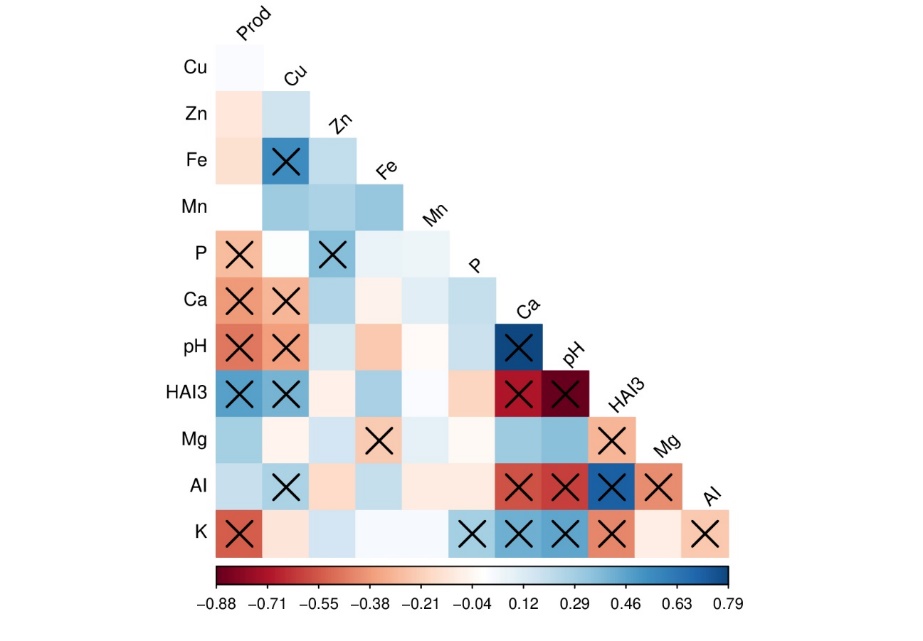
Figure 1. shows Pearson's linear correlation values between soil chemical attributes and yield.
Figure 1. Pearson's linear correlation matrix, in which correlation cells marked with X indicate Pearson liner correlation values significant at 5% probability. In this figure, X indicates which linear correlation values are significant at 5% probability, and the first column indicates the linear correlations of our soybean yield (Prod) interest variable with the covariables.
The linear correlation values considered significant with yield were phosphorus (P), calcium (Ca), pH, Potential Acidity (HAI3) and potassium (K), with values of -0.28, -0.37, -0.46, 0.48 and -0.53, respectively, characterized as weak linear correlations we have (P and CA) and as moderate linear correlation (pH, HAI3 and K) according to (Gomes, 2009). The correlations indicate that excessive levels of K and Fe can have a negative impact on soybean yield, consistent with the findings of Raij et al. (2001) regarding nutrient balance in tropical soils.
Model performance using soil chemical variables
Table 2 shows the results of the analysis 1, where the RF algorithm presented the lowest RMSE (0.568) and also the highest R 2 = 0.724 , on average, that indicates that approximately 73% of soybean yield variation is explained by the chemical soil attributes.
Table 2. Results of the first analysis.
| RF | GBM | SVR | KNR | ANN | |
|---|---|---|---|---|---|
| RMSE | 0.568 | 0.651 | 0.580 | 0.806 | 0.649 |
| R2 | 0.724 | 0.634 | 0.703 | 0.430 | 0.493 |
Source: Data generated by the researcher (2024). RF: random forest, GBM: generalized boosted regression modeling, SVR: support vector regression, KNR: K-nearest neighbors regressor, ANN: Artificial Neural Networks.
Similar performances of Random Forest have been reported in yield prediction studies, confirming its robustness when dealing with complex and non-linear data relationships (Benos et al., 2021).
This trend aligns with the findings of Fan et al. (2022), who demonstrated that the integration of soil-related variables into ML models significantly enhances soybean yield prediction accuracy, particularly under varying climatic conditions
In summary, the nonparametric Mann-Whitney test applied to the RMSE values showed that most algorithm pairs presented statistically significant differences at the 5% probability level (p < 0.05) between the predicted mean values. Only the comparisons between RF and SVR, as well as between GBM and ANN, did not show significant differences at the same probability level (p > 0.05) (Mann and Whitney, 1947). See Table 3 for detailed p values obtained from the Mann-Whitney U test of the first analysis.
‘
Table 3. Pairwise p-values from the Mann–Whitney U test from the first analysis.
| GBM | SVR | KNR | ANN | |
|---|---|---|---|---|
| RF | 6.53 × 10⁻¹⁰ | 0.414 | 1.45 × 10⁻¹¹ | 5.02 × 10⁻⁷ |
| GBM | - | 1.45 × 10⁻¹¹ | 1.45 × 10⁻¹¹ | 0.253 |
| SVR | - | - | 1.45 × 10⁻¹¹ | 2.00 × 10⁻⁶ |
| KNR | - | - | - | 1.45 × 10⁻¹¹ |
Source: Data generated by the researcher (2024). RF: random forest, GBM: generalized boosted regression modeling, SVR: support vector regression, KNR: K-nearest neighbors regressor, ANN: Artificial Neural Networks.
Therefore, the models that presented a better performance for the data available in the analysis 1 were RF and SVR. RF was analyzed because between the two best models, the latter presented the lowest RMSE and the highest R2. In this model (RF), we have as the most important variables Fe and K content in the soil as shown in Figure 2, whose chart on the left shows the percentage increase in the mean quadratic error (% IncMSE), that is, it indicates how much increase exists in the mean quadratic error if the variable is removed from the model.
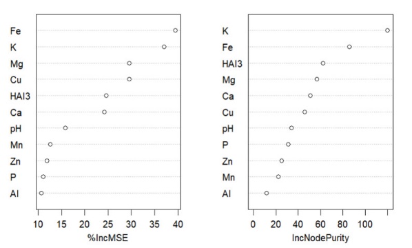
Figure 2. Variables that increase the percentage of mean squared error if removed (%IncMSE) and purity of nodes in forest decision trees (IncNodePurity) in the first analysis.
In this same figure on the right, we have the chart of purity of the decision trees nodes (IncNodePurity), which is a metric that evaluates the importance of variables by improving the nodes purity (measure of data homogeneity in a node), resulting from the division of data, and which constitute the random forest. Therefore, the K and Fe content in the soil is responsible for higher purity, meaning that the decisions made in the nodes are more discriminatory, so they are more important for the model.
Model performance including rainfall variables
Table 4 shows the results of the second analysis that includes the rainfall data accumulated in the months between sowing and harvesting, where the RF and KNR algorithms presented the lowest RMSE on average and also the highest R 2 practically, followed by the GBM algorithm.
| RF | GBM | SVR | KNR | ANN | |
|---|---|---|---|---|---|
| RMSE | 0.446 | 0.492 | 0.511 | 0.468 | 0.550 |
| R2 | 0.824 | 0.788 | 0.771 | 0.806 | 0.609 |
Table 5. Results of the second analysis.
Source: Data generated by the researcher (2024). RF: random forest, GBM: generalized boosted regression modeling, SVR: support vector regression, KNR: K-nearest neighbors regressor, ANN: Artificial Neural Networks.
The Mann–Whitney U test revealed statistically significant differences (p < 0.05) among most algorithm pairs (see Table 5). Only the comparisons between GBM and SVR, GBM and ANN, and SVR and ANN did not show significant differences (p > 0.05). These results indicate that the inclusion of rainfall data altered the relative performance of the algorithms compared to the first analysis.
Table 6. Pairwise p-values from the Mann–Whitney U test from the second analysis.
| GBM | SVR | KNR | ANN | |
|---|---|---|---|---|
| RF | 1.13 × 10⁻⁶ | 7.37 × 10⁻⁹ | 2.83 × 10⁻² | 5.02 × 10⁻⁷ |
| GBM | - | 0.211 | 5.95 × 10⁻⁴ | 0.085 |
| SVR | - | - | 4.12 × 10⁻⁶ | 0.277 |
| KNR | - | - | - | 1.83 × 10⁻⁵ |
Source: Data generated by the researcher (2024). RF: random forest, GBM: generalized boosted regression modeling, SVR: support vector regression, KNR: K-nearest neighbors regressor, ANN: Artificial Neural Networks.
Soon, RF was analyzed because between the two best models, the latter presented the lowest RMSE and the highest R2. Figure 4 shows the most important variables in the RF model.
In this analysis, the most important variables for the model were Prec_FEV and Prec_Out, which correspond to the amount of rain in the harvest months and after sowing, respectively, as shown in the variable importance plots of the RF model (Figure 3).
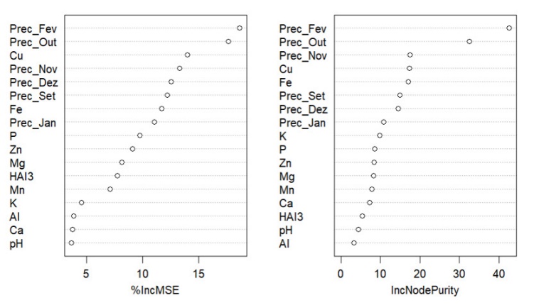
Figure 3. Variables that increase the percentage of mean squared error if removed (%IncMSE) and purity of nodes in forest decision trees (IncNodePurity) in the second analysis.
Both appear in the first positions of the percentage increase chart in the mean quadratic error of removed variables and in the purity chart of the decision tree nodes. The relevance of these rainfall variables for yield prediction is consistent with the findings of Carmello and Neto (2016), who reported that irregular rainfall during the reproductive phase significantly affects soybean productivity in southern Brazil, and also with the results of Gasparin et al. (2024), who observed a similar effect, relating excessive rainfall during harvest months to reductions in grain yield.
Visualization of results and agronomic interpretation
Figure 4 shows the soybean yield surfaces, due to the two most important chemical attributes.
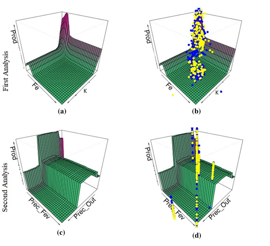
Figure 4. Surfaces of the most important variables in relation to productivity in the first and second analysis.
Maps (a) and (b) bring the most important variables in the first analysis, potassium content (K) and iron content (Fe). It is observed that the increase of these chemical elements in the soil ends up being detrimental to yield. Whereas in maps (c) and (d), the most important variables in the second analysis were precipitation in February and precipitation in October. It is also noted that a high rain in these months becomes harmful to soybean yield. Maps (b) and (d) show the training set points in blue and the points of the test set in yellow, respectively, for each analysis.
Iron (Fe) and potassium (K) contents were harmful to soybean yield, as observed in Table 1. The average Fe content was 40.09 mg dm⁻³, and the average K content was 0.44 cmolc dm⁻³, which are considered good and very high, respectively, according to the soil fertility and plant nutrition classification proposed by Raij et al. (2001).
Model validation and implications for precision agriculture
The RF models that were the best among the algorithms in analyses 1 and 2 were saved as RF1 and RF2. To exemplify the results, both models were applied to predict the 2022/2023 harvest. The results are illustrated in sequence in Figure 5 that presents the Post-Plot of Predicted Productivity in the 1st Analysis (a), Post- Plot of Predicted Productivity in the 2nd Analysis (b), Post-Plot of real yield of the year-harvest 2022/2023 (c), Post-Plot of real yield difference and predicted in the 1st Analysis (d) and Post-Plot of real yield difference and predicted in the 2nd analysis (e).
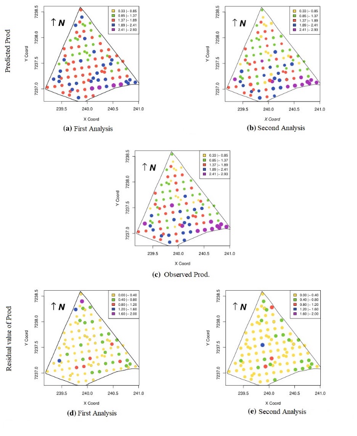
Figure 5. Post-Plots of observed, predicted and residual value productivity for the two analyses of the 2022/2023 crop year.
We can observe that between the predicted yield in the two analyzes, the one predicted by the second model presented a Post-Plot (b) closer to the real (c), while the Post-Plot (a) presents a difference mainly in the low production points, which are represented in yellow in the Post-Plot (c). Thus, Post-Plot (d) ends up having higher difference values than Post-Plot (e).
The enhanced agreement between predicted and observed yield indicates that incorporating climatic variables improves the robustness of ML models under real production conditions, as also highlighted by Benos et al. (2021).
Figure 6 shows scatterplots comparing Actual Yield for Crop Year 22/23 (x-axis) with Predicted Yield (y-axis) in both analyses.
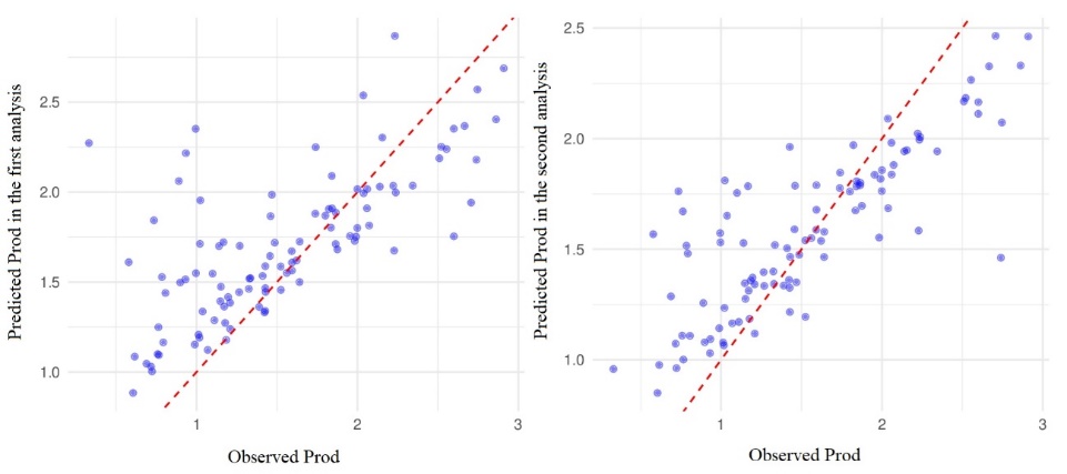
Figure 6. Scatter plots of observed versus predicted productivity: on the left, the first analysis; on the right, the second analysis. The dashed line represents the 1:1 line.
It is noted that the model of the second analysis had an improvement in the adjustment in relation to that of the first one, since the points are closer to the red line. This improvement suggests a greater model accuracy of the second analysis.
Materials and Methods
Area under study and dataset
The study area of 167.35 hectares is located in the municipality of Cascavel Figure 7, in the western region of Paraná, Brazil. It is a commercial area of production of soybean and corn grains with no-tillage, with approximate geographic coordinates of latitude and longitude of 24.95 South and 53.3-7 West and 650 meters of average altitude. The climate of the region is mesothermic and superhumid, a climate of the type Cfa (Koeppen), with an annual average temperature of 21ºC and a typical Dystroferric Red Latosol with a clayey texture (Santos et al., 2018). The average slope of approximately 4%, categorized as smooth wavy.
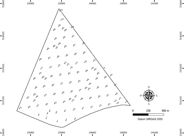
Figure 1. Study area, in which each numbered point corresponds to a sample. Source: Spatial Statistics Laboratory - UNIOESTE.
In the data collection, 102 sampling points were determined using the lattice plus close pairs technique, which allows a uniform distribution of sampling points in the study area (Maltauro et al., 2023a). This drawing contains a regular grid with 83 points (with a distance of 141 meters between the points) and in addition to these points, 19 points were added randomly with restriction that these new sampling points would have a maximum distance of 50 and 75 meters from the regular grid points. The sample was georeferenced and localized with the support of a signal receptor device with Global Positioning System (GPS) configured for the Universal Transverse Mercator (UTM) coordinate system of the Spatial Statistics Laboratory of the Universidade Estadual do Oeste do Paraná - UNIOESTE, Cascavel - PR.
Information on soybean yield, soil chemical properties and accumulated monthly rainfall of 7 crop years (2012/2013, 2013/2014, 2014/2015, 2015/2016, 2019/2020, 2021/2022, 2022/2023) with 102 observations Figure 1 for each year, generating a total of 714 observations.
Soybean yield was collected based on the amount of grains harvested from plants distributed in two lines, along one meter length of each point, representing the plot. After sorting, the grains were weighed for each plot, checking the water content and correcting for 13% moisture, and then converted into t ha⁻¹.
For the prediction of soybean yield (Prod, t ha⁻¹), the following chemical properties of the soil were used as covariates: copper content (Cu, mg dm⁻³), zinc content (Zn, mg dm⁻³), iron content (Fe, mg dm⁻³), manganese content (Mn, mg dm⁻³), phosphorus content (P, mg dm⁻³), calcium content (Ca, mg dm⁻³), magnesium content (Mg, cmolc dm⁻³), aluminum content (Al, cmolc dm⁻³), potassium content (K, cmolc dm⁻³), pH, and potential acidity (H⁺ + Al³⁺, cmolc dm⁻³). Information on the collection methodology for soil laboratory analysis for this agricultural area is described by Maltauro et al. (2023a) and Maltauro et al. (2023b).
It was also considered as covariable with the accumulated monthly precipitation (mm) in the study area. The months considered in the calculation of monthly accumulated precipitation were: September (Prec_Set), October (Prec_Out), November (Prec_Nov), December (Prec_Dec), January (Prec_Jan) and February (Prec_Feb) which are the months of the soybean cycle, from sowing to harvest. Precipitation data were obtained from the NASA Langley Research Center (LARC) Prediction of Worldwide Energy Resources (POWER) Project, funded by NASA’s Earth Science/Applied Science Program (NASA LARC, 2024).
Thus, two analyzes were made, one with only soil chemical properties, being the predictive or covariable variables (analysis 1) and another analysis including the accumulated monthly precipitation in the predictive variables (analysis 2). The missing data were replaced by the average of their variable in the corresponding harvest year. Initially, an exploratory study of the variables was carried out and Pearson's linear correlation was calculated between the pairs of variables in the dataset.
Machine Learning Models
For the yield prediction the models described below were used, whose equations are described in Table 7.
Table 1. Machine learning models.
| Model | Equation |
|---|---|
| RF | \[\widehat{Y} = \frac{1}{N}\sum_{i = 1}^{N}{f_{i}(X)}\] |
| GBM | \[\widehat{Y} = Y_{0} + \sum_{i = 1}^{N}{{\alpha_{i}f}_{i}(X)}\] |
| SVR | \[\widehat{Y} = \sum_{i = 1}^{N}{\beta_{i}Ke\left( X,\ X_{i} \right) + b}\] |
| KNR | \[\widehat{Y} = \frac{1}{K}\sum_{j = 1}^{K}y_{j}\] |
| ANN | \({\widehat{Y}}_{\mathbf{i}}^{(\mathbf{v})} = g^{(\mathbf{v})}\left( \sum_{i = 1}^{N}{w_{i}^{(v)}{\widehat{Y}}_{i}^{(v - 1)} + b^{(v)}} \right)\), com \({\widehat{Y}}_{i}^{(0)} = X_{i}\) |
\(\widehat{Y}\): predicted value of modelo; \(N\): number of trees; \(f_{i}(X)\): prediction of the i-th tree for input X, with \(i = 1,\ \ldots,\ N\); \(Y_{0}\): initial prediction value; \(\alpha_{i}\): learning rate associated with the correction applied by the i-th tree; \(\beta_{i}\): Lagrange coefficient; \(Ke\left( X,\ X_{i} \right)\): Radial Kernel function that calculates the inner product between \(X\) and \(X_{i}\); \(b\): regression hyperplane intercept; \(K\): number of nearest neighbors; \(y_{j}\): value of the response variable in the j-th instance, with \(j = 1,\ \ldots,\ K\); \(w_{i}^{(v)}\): weight of the v-th layer associated with the i-th input, with \(v = 1,\ \ldots,\ M\) and \(i = 1,\ \ldots,\ N\); \(M\): number of layers in the neural network; \(g^{\left( \mathbf{v} \right)}( \bullet )\): activation function of neurons in the v-th layer; \(b^{(v)}\): v-th layer bias; \(X_{i}\): initial input.
Random Forest (RF) is a ML technique that belongs to the ensemble method category. It combines the forecasts of several individual decision trees to produce a more robust and general prediction. Each tree is trained in a random sample of the dataset and uses only a random subset of the available resources. This introduces diversity into individual trees and reduces the correlation between them. The main idea behind RF is to reduce the variance of training data while keeping bias low. This means that the model becomes less sensitive to changes in training data. At the same time, it maintains a low bias, ensuring that the model does not become overly simplified, resulting in a more robust model and less prone to overfitting (Breiman, 2001).
The final RF prediction is obtained by combining the forecasts of all individual trees and their general equation is described in Table 1 (Breiman, 2001). For this study, the number of trees (N) was set to 500, as the error curve indicated that this value was sufficient to stabilize the model; after this point, the gains became marginal. The number of variables considered at each split (mtry) followed the default value suggested by Hastie et al. (2009), which is the total number of variables divided by three. The importance of the variables (importance) was pre-defined as true, which allows us to evaluate which variables are most influential in the model. The aforementioned authors presented a detailed analysis of the RF method, highlighting its predictive power and its ability to deal with a wide range of ML problems.
The Generalized Boosted Regression Modeling (GBM) algorithm, an extension of the boosting algorithm originally proposed by Freund and Schapire (1996), is widely used in machine learning problems, especially in regression tasks. GBM builds a robust predictive model from a simpler set of models, sequentially, adjusting the observations weights based on the performance of the previous model, prioritizing those that contribute most to residual errors. This approach allows the model to focus on the most challenging instances of predicting, gradually improving predictive performance with the aim of minimizing the overall error of the combined model.
The final GBM model, whose general equation is described in Table 1, is an initial prediction plus the addition of the contribution of weak models (Hastie et al., 2009). During the GBM training, the fi(x) trees are adjusted to capture the residual errors of the previous model (Friedman, 2001).
For this study, the following GBM parameters were used: the initial forecast value was considered as the mean of the response variable values; the distribution of errors (distribution) was defined as Gaussian, appropriate for regression problems (Kuhn and Johnson, 2013); the number of trees (N) was defined as 2000, the sampling fraction (bag.fraction) defined as 0.5, and means that each tree will be trained with 50% of the randomly selected samples with replacement, this helps to reduce the model variance (James et al., 2013); the interaction depth (interaction.depth) was defined as 1, meaning that each tree is a simple linear regression model (HASTIE et al.,2009); and the learning rate (shrinkage, αi, i = 1, ..., N ) has been defined as 0.1, (smaller values make training slower) controlling the contribution of each tree in the sequence and helping to avoid overfitting (James et al.,2013).
Support Vector Regression (SVR) is a machine learning technique used to perform regression, i.e. predict continuous values based on a training dataset. SVR is an extension of Support Vector Machines (SVMs) for regression problems (Smola and Schölkopf, 2004).
The SVR approach is to find a regression function, f(x) = \(\widehat{Y}\) that approaches the training data with the lowest possible margin of error, while keeping this margin within a user-controlled limit (Cortes and Vapnik, 1995). The SVR prediction function is described in Table 1 (Hastie et al., 2009).
The coefficients αi and the term b are adjusted by solving an optimization problem that minimizes a cost function, subject to restrictions that ensure that errors within a specified margin are not penalized, that is, the errors within this margin are not penalized, helping to create a more robust model (Vapnik, 1995; Schölkopf and Smola, 2002). During the SVR training, the cost parameter was defined as 1, thus controlling between having a low training error model and a wide decision margin model (Steinwart and Christmann, 2008).
The K-Nearest Neighbors Regressor (KNR) method was initially proposed by Fix and Hodges (1951) for classification, and its application in regression problems is discussed in Bishop (2006). KNR shows itself a powerful and intuitive machine learning technique to solve regression problems. This learning model is particularly useful in situations where the relationship between attributes and output is not easily modeled by a parametric function (Hastie et al., 2009).
It is an example of an instance-based algorithm, where learning is performed directly from the training set, and in this method, the prediction for a new instance is made considering the target values of the closest known K instances in the attribute space. To perform a forecast with KNR, we first identified the closest K neighbors to the new instance in the training set using Euclidean distance (Hastie et al., 2009). The predictive variables are essential in this process, because they are used to calculate the distances between the new instance and the instances of the training set; thus, determining the nearest K neighbors. Although crucial in this process, they do not appear explicitly in the prediction equation, which is calculated as the mean (or other aggregating function) of the target values of the nearest K instances (Table 1) (Hastie et al., 2009). The choice of K value is crucial, as it determines the smoothness of the decision border and the model complexity (Bishop, 2006). For the implementation of KNR, the following parameters were used, the method to be used (method) defined as KNN, which was chosen for its simplicity and effectiveness in many regression problems (Hastie et al., 2009). For the training control we used Cross Validation (VC) with 10 folds since 10 is an adequate value for the stability of the second model estimate (James et al., 2013). The K value was automatically adjusted during the training process and chosen for the best performance of the evaluation metrics obtained by cross-validation.
Artificial Neural Networks (ANNs) are computational models inspired by the structure and functioning of the biological nervous system, specifically the human brain (Goodfellow et al., 2016). According to Bishop (2006), an ANN is composed of simple processing units called neurons, arranged in layers. The input layer receives the input data, the output layer produces the final results, and the intermediate layers, called hidden layers, process the information between the input and output.
The functioning of an ANN is based on mathematical operations performed on each neuron. Each neuron receives weighted inputs, performs a weighted sum of these inputs and applies an activation function to produce output (Table 1) (Nielsen, 2015; Aggarwal, 2018). The initial bias value is randomly defined and adjusted during neural network training. The g-activation function applied to each neuron, introduces non-linearity in the network and allows it to learn complex relationships in the data, applied after the weighted sum of the inputs and weights plus the bias term. The following activation functions were tested: identity, logistics, hyperbolic tangent and ReLU.
ANNs learn by adjusting weights and bias during training, using optimization algorithms such as the downward gradient to minimize a loss function that quantifies the error between the outputs predicted by the network and the actual values of the training data. They are widely used in areas such as pattern recognition, natural language processing, computer vision, among others, due to their ability to learn and generalize from data.
To validate the best adjusted model in each methodology the mean root statistics of the square average error (RMSE) and the mean of the coefficient of determination(R2) were used after running 20 times each algorithm separating the data in 2/3 for training and 1/3 for random testing (Goodfellow et al., 2016). The Mann and Whitney U test (1947) was applied to pair with models to verify if there are significant differences at a level of 5% between the RMSE values groups of each algorithm. The model with the lowest RMSE and the largest R 2 was selected. All computational implementation was done in R (R Core Team, 2024) software version 4.3.3, using the randomForest packages (Liaw and Wiener, 2002), gbm (Greenwell et al., 2022), e1071 (Meyer et al., 2023), class (Venables and Ripley, 2002) and caret (Kuhn, 2022).
Conclusion
The results of this study show that the Random Forest (RF) model was especially promising in predicting soybean yield when using soil chemical attributes. By including the rainfall variables accumulated during the months of the soybean cycle, the RF model showed an improvement in the evaluation metrics. These adjustment gains in the model have important implications for farmers, allowing them to make more informed decisions, optimize the use of their resources, and plan their crops more accurately. In addition, the analysis highlights the importance of using machine learning as a crucial tool in the analysis of agricultural data, which can be replicable in other areas of study. This highlights the importance of exploring and applying machine learning techniques to advance the understanding of complex dynamics in agricultural environments, allowing a more detailed and accurate analysis, and contributing to innovation and sustainability in agriculture.
Acknowledgements
We are thankful to the support of the Coordination for the Improvement of Higher Education Personnel - CAPES, funding code 001, CNPq and Applied Statistics Laboratories (LEA), Spatial Statistics (LEE) and the postgraduate program in agricultural engineering (PGEAGRI) both belonging to Universidade Estadual do Oeste do Paraná - UNIOESTE.
References
Aggarwal CC (2018) Neural networks and deep learning: a textbook. New York: Springer.
Akhter R, Sofi SA (2022) Precision agriculture using IoT data analytics and machine learning. J King Saud Univ Comput Inf Sci 34:5602–5618.
Baerdemaeker JD (2013) Precision agriculture technology and robotics for good agricultural practices. IFAC Proc 46(4):1–4.
Benos L, Tagarakis AC, Dolias G, Berruto R, Kateris D, Bochtis D (2021) Machine learning in agriculture: a comprehensive updated review. Sensors 21:358.
Bernardi ADC, Bettiol GM, Grego CR, Andrade RG, Rabello LM, Inamasu RY (2015) Ferramentas de agricultura de precisão como auxílio ao manejo da fertilidade do solo. Cienc Tecnol 32(1/2):211–227.
Bishop CM (2006) Pattern recognition and machine learning. New York: Springer.
Breiman L (2001) Random forests. Mach Learn 45:5–32.
Carmello V, Neto JLS (2016) Rainfall variability and soybean yield in Paraná State, southern Brazil. Int J Environ Agric Res 2(1):86–97.
Chlingaryan A, Sukkarieh S, Whelan B (2018) Machine learning approaches for crop yield prediction and nitrogen status estimation in precision agriculture: a review. Comput Electron Agric 151:61–69.
Conab (2024) Acompanhamento da safra brasileira de grãos. 12ª ed. Brasília: Companhia Nacional de Abastecimento. Disponível em: https://www.conab.gov.br/info-agro/safras
Cortes C, Vapnik V (1995) Support-vector networks. Mach Learn 20:273–297.
Fan J, Liu Y, Xu R, Zhang X (2022) Soybean yield prediction by machine learning and climate. Theor Appl Climatol 149(3–4):1079–1093.
FAO (2018) Food and agriculture organization of the United Nations. Disponível em: http://www.fao.org
Fiss G, Schuch LOB, Peske ST, Castellanos CIS, Meneghello GE, Aumonde TZ (2018) Produtividade e características agronômicas da soja em função de falhas na semeadura. Rev Cienc Agrar Amaz J Agric Environ Sci 61:1–7.
Fix E, Hodges JL (1951) Discriminatory analysis, nonparametric discrimination: consistency properties. USAF School of Aviation Medicine, Randolph Field, Texas.
Freund Y, Schapire RE (1996) Experiments with a new boosting algorithm. In: Proc 13th Int Conf Mach Learn (ICML’96).
Friedman JH (2001) Greedy function approximation: a gradient boosting machine. Ann Stat 29:1189–1232.
Gao H (2021) Agricultural soil data analysis using spatial clustering data mining techniques. In: Proc IEEE 13th Int Conf Comput Res Dev (ICCRD). p. 83–90.
Gasparin PP, Da Silva EM, Becker WR, Paludo A, Guedes LPC, Johann JJ (2024) Agroclimatic and spectral regionalization for soybean in different agricultural settings in the State of Paraná, Brazil. J Agric Sci 1–16.
Gelain E, Bottega EL, Motomiya AVA, Oliveira ZB (2021) Variabilidade espacial e correlação dos atributos do solo com produtividade do milho e da soja. Nativa 9(5):536–543.
Gomes FP (2009) Curso de estatística experimental. 15ª ed. Piracicaba: FEALQ.
Goodfellow I, Bengio Y, Courville A (2016) Deep learning. Cambridge: MIT Press.
Hastie T, Tibshirani R, Friedman J (2009) The elements of statistical learning: data mining, inference, and prediction. 2nd ed. New York: Springer.
James G, Witten D, Hastie T, Tibshirani R (2013) An introduction to statistical learning: with applications in R. New York: Springer.
Khaki S, Wang L (2019) Crop yield prediction using deep neural networks. Front Plant Sci 10:621.
Liakos KG, Busato P, Moshou D, Pearson S, Bochtis D (2018) Machine learning in agriculture: a review. Sensors 18(8):2674.
Kuhn M, Johnson K (2013) Applied predictive modeling. New York: Springer.
Maltauro TC, Guedes LPC, Uribe-Opazo MA, Canton LE (2023a) Multivariate spatial sample reduction of soil chemical attributes by means of application zones. Span J Agric Res 21(2):e0205.
Maltauro TC, Guedes LPC, Uribe-Opazo MA, Canton LE (2023b) Otimização multivariada espacial para um redesenho de amostragem com tamanho de amostra reduzido de propriedades químicas do solo. Rev Bras Cienc Solo 47:e0220072.
Mann HB, Whitney DR (1947) Test for randomness against a specified alternative. Econometrica 13:245–259.
NASA Langley Research Center (LARC) (2024) NASA Prediction of Worldwide Energy Resources (POWER) Project. NASA Earth Science/Applied Science Program. Available at: https://power.larc.nasa.gov
Nielsen MA (2015) Neural networks and deep learning. Determination Press.
Payton ME (1996) Confidence intervals for the coefficient of variation. Commun Stat Simul Comput 25:159–174.
Raij BV, Andrade JC, Cantarella H, Quaggio JA (2001) Fertilidade do solo e nutrição de plantas. Campinas: Instituto Agronômico.
Santos HG, Jacomine PKT, Anjos LHC, Oliveira VA, Lumbreras JF, Coelho MR, Almeida JA, Filho JAA, Oliveira JB, Cunha TJF (2018) Sistema brasileiro de classificação de solos. 5ª ed. Brasília: Embrapa.
Schölkopf B, Smola AJ (2002) Learning with kernels: support vector machines, regularization, optimization, and beyond. Cambridge: MIT Press.
Smola AJ, Schölkopf B (2004) A tutorial on support vector regression. Stat Comput 14:199–222.
Steinwart I, Christmann A (2008) Support vector machines. New York: Springer.
Vapnik VN (1995) The nature of statistical learning theory. New York: Springer.
Veeragandham S, Santhi H (2020) A review on the role of machine learning in agriculture. Scalable Comput Pract Exper 21(4):583–589.
Venables WN, Ripley BD (2002) Modern applied statistics with S. New York: Springer.
Wolfert S, Ge L, Verdouw C, Bogaardt MJ (2017) Big data in smart farming: a review. Agric Syst 153:69–80.
Zipper SC, Qiu J, Kucharik CJ (2016) Drought effects on US maize and soybean production: spatiotemporal patterns and historical changes. Environ Res Lett 11:094021.